Item Response Theory Calibration and Linking: Establishing a Common Measurement Scale Across Samples, Forms and Time

1. Introduction

Item response theory places persons and items on one latent continuum, but the origin and unit of that continuum are not fixed by the model. Any linear transformation of the latent variable, accompanied by the matching transformation of the item parameters, leaves every response probability unchanged (Lord, 1980; Embretson & Reise, 2000; Oladunmoye & Muhammad , 2024; Oladunmoye, 2015). A calibration therefore returns parameters on a scale defined by whatever constraint the analyst or software imposed, usually a standard normal distribution for the calibration sample. Two calibrations that each impose this constraint on different samples do not share a scale, even though both are standardised.

The consequence is easy to overlook. Suppose an item has a difficulty of 1.20 in one calibration and 0.85 in a later one. The item may have become easier, the second sample may be more able, the second calibration may have used a different unit, or all three may be true. The difference alone cannot distinguish between these explanations. Separating them needs a procedure that connects the two scales, and that procedure is called linking.

The problem has grown with the spread of item banks, computerised adaptive testing (Wainer et al., 2000; van der Linden & Glas, 2010), patient-reported outcome systems built on a reference metric (Reeve et al., 2007; Choi et al., 2014), longitudinal designs, and the adaptation of instruments across languages and cultures. In each setting items and samples accumulate over calibration waves, and every wave must be placed on one metric if the bank is to remain coherent.

The literature has not always been consistent about what linking is. Standard treatments present it as a step within test equating (Holland & Dorans, 2006; Kolen & Brennan, 2014; Oladunmoye, Enamudu,, Ogbu, 2024). van der Linden and Barrett (2016) argue instead that parameter linking arises from the non-identifiability of the latent metric and is needed whether or not number-correct scores are ever equated. A third idea, measurement invariance, is sometimes conflated with both.

This study has four aims: to separate calibration, linking, equating and invariance; to review designs, calibration strategies and transformation methods, correcting common errors of convention; to show by Monte Carlo illustration how the methods behave under anchor drift, how large linking error is relative to sampling error, and how error accumulates along chains; and to propose reporting standards and a record-keeping architecture for item banks, with the PsychtrixWeb platform as the applied setting. It builds on earlier notes in this series on differential item functioning (DIF), invariance, adaptive testing and item banking (Oladunmoye, 2026 a,b,c).

2. Calibration, indeterminacy and the logic of linking

2.1 Why separate calibrations do not share a scale

Consider the two-parameter logistic (2PL) model, in which the probability that a person with latent trait θ answers item i in the keyed direction is

(1)

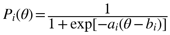
where a_i is the discrimination and b_i the location (difficulty) of the item. Calibration is the estimation of these parameters, and of population parameters where they are modelled, from one response dataset under one model. Now let θ* = Aθ + B with A > 0. Because a_i(θ − b_i) = (a_i/A)[θ* − (Ab_i + B)], the response probabilities are unchanged if the scale and the item parameters are transformed together:

(2)

(3)

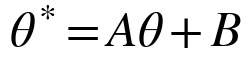
A governs the unit and B the origin. Estimation software removes the indeterminacy by constraint, most often by fixing the ability distribution of the calibration sample at mean 0 and variance 1 (in Rasch calibrations, by fixing the mean item difficulty). The constraint is a convention applied within a sample. If a second sample differs in mean or spread, the same item receives different parameters in the two runs for reasons unrelated to the item. Standardising both calibrations therefore does not make them equivalent, a point that van der Linden and Barrett (2016) derive formally for monotone response models.

Figure 1 illustrates the point with the example above. Item X has a = 1.20 and b = 0.50 in calibration A and a = 1.05 and b = 0.20 in calibration B. With A = 0.875 and B = 0.325, so that θ_A = 0.875θ_B + 0.325, the two sets of parameters describe the same item characteristic curve. The example also shows a limit of single anchors. Any one item can be reconciled exactly by some choice of A and B, so evidence of genuine change can appear only as inconsistency across several items.

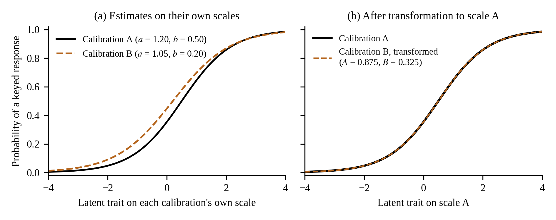
Figure 1. The same item expressed on two calibration scales. (a) Estimates as reported by each calibration. (b) Calibration B after transformation to scale A with θ_A = 0.875θ_B + 0.325.

2.2 Calibration, linking, equating and invariance

Four terms need to be kept apart (Table 1). Calibration estimates parameters within one dataset. Linking expresses parameters from different calibrations on one metric. Equating is a further operation on scores: it aims to make scores from different forms interchangeable, which requires that the forms measure the same construct with similar reliability and that the conversion does not depend on the population used (Holland & Dorans, 2006; Kolen & Brennan, 2014; Oladunmoye, Enamudu,& Sa'ad, 2024). Invariance is a property of the measurement model rather than an operation, and it asks whether items function equivalently across groups or occasions (Meredith, 1993; Millsap, 2011; Oladunmoye, Agbor, Olabisi, & Oyadeyi, 2024).

Table 1. Four related but distinct concepts.

The relationships are directional. Linking can be done without equating, for example when a bank is placed on one metric and each person is scored with whichever items they received. Equating presupposes a link between forms, and IRT true-score equating, which converts number-correct scores through test characteristic curves, uses parameters that have first been placed on a common metric. Invariance enters from the other side. A link built on non-invariant anchors is biased, and a linked metric says nothing by itself about whether the construct means the same in two groups. Linking can secure statistical comparability (the parameters share a mathematical scale) and metric comparability (the same number denotes the same latent location). Substantive comparability (the construct keeps its meaning) and interpretive comparability (scores may legitimately be read alike) depend on invariance and validity evidence of a different kind.

3. Data collection designs and calibration strategies

3.1 Designs

The empirical connection between calibrations comes from shared items, shared persons, or randomly equivalent groups. In the common-item design, known in the equating literature as the nonequivalent groups with anchor test (NEAT) design, different groups take different forms that contain a set of common items. The anchor separates differences between groups from differences between forms, because the groups can be compared on items both answered (Kolen & Brennan, 2014). Observed-score equating methods in this design rest on assumptions about the data that are missing by design, and the methods can give different answers when those assumptions fail (Sinharay & Holland, 2010). IRT linking replaces those assumptions with a parametric model and the assumption that the anchor items behave in the same way in both groups.

In the common-person design the same examinees answer both item sets. This gives a direct person-level connection and suits small item pools, but it is exposed to order, practice and fatigue effects and, where the interval between administrations is long, to genuine change in the persons, which then cannot be separated from change in the metric. In the equivalent-groups design examinees are randomly assigned to forms and the groups are treated as equal in the latent trait. No common items are needed, but the link then offers no way to check whether items behave identically. Designs can be combined, and shared items together with shared persons give the most information for a given burden.

3.2 Calibration strategies

Given a design, parameters can be placed on a common scale in three broad ways. In separate calibration, each dataset is calibrated alone and a transformation estimated from the shared items is applied afterwards. In concurrent calibration, all data are estimated in one run. In a NEAT design this requires a multiple-group model in which each group has its own ability distribution (Bock & Zimowski, 1997), since a single-group run would treat the groups as equivalent. In fixed-parameter calibration, the shared items are held at previously established values while new items are estimated, which keeps the new items on the existing metric by construction.

Evidence on the relative merits is mixed and depends on conditions. Kim and Cohen (1998) found that characteristic-curve linking gave smaller root mean square differences than concurrent calibration when few common items were available, and that the approaches converged as common items increased. Hanson and Béguin (2002) found that concurrent estimation generally produced lower error but not universally, and they cautioned against abandoning separate estimation. Fischer et al. (2021) studied small item pools under the Rasch model and reported convergence problems for concurrent calibration, while the other methods recovered parameters adequately. Fixed-parameter calibration is widely used to maintain banks, but implementations differ and affect results (Kim, 2006). Because the anchors are held fixed, any drift in them passes silently into the new items unless a free calibration is run as a check. Separate calibration has the practical advantage that the behaviour of each anchor in both samples can be inspected before the transformation is applied, and it is the default in the illustration of Section 7.

4. Transformation methods

Under separate calibration the linear transformation can be estimated in four common ways (Table 2). Write the transformation as θ_t = Aθ_s + B, where the source scale s is the calibration to be transformed and the target scale t is the reference. Item parameters then transform as in Equation 3, so that b_t = Ab_s + B and a_t = a_s/A. The inverse transformation, θ_s = θ_t/A − B/A, has constants 1/A and −B/A. Constants reported without a stated direction leave the reader unable to tell which of the two was meant, and textbooks and software do not use a single convention. Reversal of the direction is a frequent source of error in applied reports.

Moment methods use the means and standard deviations of the anchor parameters. The mean-sigma method (Marco, 1977) uses the difficulty parameters,

(4)

and the mean-mean method (Loyd & Hoover, 1980) takes the unit from the discrimination parameters,

(5)

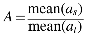
with B from the difficulty means as before. Both are simple and transparent, but both weight every anchor equally, ignore the precision of individual estimates, and are sensitive to outlying items. Mean-sigma also becomes unstable when the anchor difficulties have little spread, because A is then a ratio of two small numbers.

Characteristic-curve methods choose A and B so that the response functions of the anchor items agree across calibrations. The Stocking-Lord method (Stocking & Lord, 1983) minimises the weighted squared difference between the test characteristic curves of the anchor set,

(6)

where P^s* is the response function of the source item after transformation and w_q are weights at quadrature points θ_q. The Haebara method (Haebara, 1980) minimises squared differences item by item,

(7)

so that a discrepancy in one item cannot be offset by an opposite discrepancy in another, as it can when curves are summed. Both criteria are often symmetrised by adding the same quantity computed in the reverse direction (Kolen & Brennan, 2014). The weights are an analytic choice rather than a fact about the data, and results can change with them.

Unifying treatments exist. von Davier and von Davier (2007) express mean-mean, characteristic-curve, concurrent and fixed-parameter approaches as restrictions on the item-parameter space of a likelihood, which makes their relationship explicit. van der Linden and Barrett (2016) derive the form of the linking function from identifiability alone, and give its specific shapes for parameterisations of the three-parameter model. When many forms are connected, the constants for all forms can be estimated simultaneously rather than pair by pair (Haberman, 2009; Battauz, 2017). No method is uniformly best, and the choice should be justified by the design and the diagnostics.

Table 2. Linking and calibration approaches: information used and main cautions.

5. Anchor quality, drift and linking error

5.1 Anchor design

The shared items carry the whole burden of the link, so their quality matters more than their number. Anchors should represent the content of the full instrument, and Klein and Jarjoura (1985) showed that content representation of common items matters for equating with nonrandom groups. Anchors should also span the part of the latent range in which the groups lie. Wingersky et al. (1987) found that longer linking sets and a uniform distribution of examinee ability improved IRT true-score equating, and that the efficiency of the linking items relative to the total test was a better guide than the size of their standard errors. A frequently quoted heuristic holds that anchors should make up at least about 20 per cent of the test (Kolen & Brennan, 2014), and a simulation with small item pools suggested that the share may need to be larger when the model fits imperfectly (Fischer et al., 2021). The heuristic is a planning starting point, not a criterion of adequacy.

5.2 Drift and differential functioning

An anchor can be well chosen and still behave differently in two calibrations. Reasons include genuine population differences (DIF), exposure or disclosure, edits to wording or translation, changes in scoring or administration context, estimation error and model misfit. The change is called item parameter drift when it occurs over time and DIF when it occurs between groups, and its effect on the link is the same. Bock et al. (1988) addressed item pool maintenance under drift, and Donoghue and Isham (1998) compared procedures for detecting it. Outlying common items can distort equating, and how they are treated changes the outcome (Hu et al., 2008; Michaelides, 2010). Candell and Drasgow (1988) proposed an iterative procedure that links on items judged unbiased, and showed that it improved bias detection over a single pass. Kopf et al. (2015) reviewed anchor selection strategies in DIF analysis, which face the mirror-image problem of needing a DIF-free anchor in order to detect DIF.

Purification carries risks of its own. Li (2012) found that excluding drifted polytomous anchors generally improved equating, but also that removal can leave an anchor that no longer resembles a miniature of the full test, which violates the content condition above. An item should therefore not be deleted merely because its estimate has moved. Movement may reflect sampling variation, genuine population differences or an inadequate transformation. Statistical flags should trigger review of content and context, and the decision and its reasons should be recorded. Section 7 gives a quantitative example of the cost of mechanical deletion.

5.3 Linking error

The constants A and B are estimates, so a linked parameter carries error from the link in addition to its own sampling error. Ignoring this is standard practice. Sheehan and Mislevy (1988) outlined how the uncertainty can be accounted for, using a jackknife approximation for Stocking-Lord linking. In their examples it was usually negligible for inferences about individuals but could be a major source of error in aggregate statistics such as changes in group means. Ogasawara (2001) derived asymptotic standard errors for response-function methods. Michaelides and Haertel (2014) showed that the particular set of common items is a further source of variability, which does not shrink as the examinee sample grows and can come to dominate error in group means. In international surveys, PISA included a linking error in the standard errors of trend estimates, whereas the IEA surveys did not at the time of the comparison by Monseur and Berezner (2007), who also proposed a replication-based alternative. Wu (2010) treats equating error alongside measurement and sampling error as the three main error sources in large-scale assessment.

Practical estimators include analytic standard errors, the jackknife, and the bootstrap, in which examinees are resampled, each calibration is repeated and the transformation re-estimated. A person-level bootstrap with items held fixed captures examinee sampling only. The contribution of anchor selection must be examined separately, for example by re-linking on random subsets of the anchor set.

5.4 Diagnostics

Transformation quality can be checked by comparing curves before and after transformation. Let T_t(θ) be the test characteristic curve of the anchor set in the target calibration and T_s*(θ) the same curve computed from the transformed source parameters. Two simple summaries over a grid θ₁, …, θ_K are

(8)

(9)

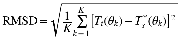
Item-level equivalents identify which anchors are responsible. Neither summary has a universal cut-off. Acceptable values depend on the model, the number of anchors, the stakes of the decision and the scale of the summary, since curves for tests are in score units and curves for single items are probabilities. Plots usually say more than the summaries: anchor curve overlays, scatterplots of target against transformed source difficulties with an identity line, residual plots, and information functions before and after linking.

6. Extensions

Polytomous and multidimensional models. For graded and partial credit models the same linear transformation applies to the latent variable, but the parameter set also contains thresholds or step parameters. Each of these is shifted and scaled like a difficulty, while discriminations are rescaled by 1/A. Treating all parameters alike is an error, and the correct rule depends on the parameterisation. Baker (1992) described equating under the graded response model (Samejima, 1969), and Haberman (2009) and von Davier and von Davier (2007) cover the generalised partial credit model (Muraki, 1992), of which the partial credit model (Masters, 1982) is a special case. In multidimensional models the transformation is θ* = Aθ + b with a matrix A and a vector b, so translation, dilation and rotation must all be identified. Oshima et al. (2000) compared practical approaches, and Reckase (2009) gives the model background.

Vertical scaling and longitudinal measurement. Vertical scaling places forms intended for different levels, such as school grades or developmental stages, on one continuum so that growth can be described. Its results depend on the design, the calibration approach and the linking method (Tong & Kolen, 2007). In longitudinal research the central problem is to separate true change from measurement change. If item parameters drift between waves, apparent change in the latent variable may be an artefact. Stable anchors across occasions, drift monitoring at every wave, and documentation of the metric version used in each analysis are the practical safeguards.

Chains and complex linkage plans. When forms are linked in sequence, A to B and B to C, the transformations compose. If θ_B = A_ABθ_A + B_AB and θ_C = A_BCθ_B + B_BC, then

(10)

The constants of a chain are products and sums of the constants of its links, and their errors accumulate. Complex plans, with many forms and several paths between them, raise the further question of how to combine indirect links. Battauz (2013) developed average equating coefficients for forms linked through different paths and derived asymptotic standard errors for chained and averaged coefficients. Battauz (2017) extended mean-mean, Haebara and Stocking-Lord methods to estimate the coefficients of all forms simultaneously. Representing a plan as a graph, with forms as nodes and shared-item sets as edges, makes weakly connected or isolated forms visible and gives the chain length to the reference scale directly.

Cross-cultural and multilingual use. A common numerical scale does not establish that a construct has the same meaning across cultures or languages. Translated anchors may differ in difficulty or connotation, response styles differ, and the construct itself may be understood differently (van de Vijver & Leung, 1997). Multilingual banks typically rely on bilingual or translated anchors and multiple-group models, and the anchors then need review for linguistic equivalence as well as statistical screening. Reporting of invariance testing varies widely in applied work (Putnick & Bornstein, 2016), which is a reason to treat linking diagnostics as one part of the evidence and not the whole. Whether common IRT scales remain stable when psychological instruments are adapted across African populations is a research question that deserves systematic study, with language, DIF, anchor stability and linking error as the main variables.

Item banks and adaptive testing. Adaptive algorithms select items by comparing item information with a provisional ability estimate, so every bank parameter must be on the same metric as that estimate (Wainer et al., 2000; van der Linden & Glas, 2010). If part of the bank sits on another metric, an algorithm aiming at an estimate of 1.5 will choose items whose difficulties do not refer to the same location, and information and exposure calculations will be wrong. The PROMIS programme illustrates the principle at scale: item banks were developed on a reference metric (Reeve et al., 2007) and legacy depression instruments were later linked to it (Choi et al., 2014).

7. Monte Carlo illustration

7.1 Design and methods

The simulation illustrates, under controlled conditions, the behaviour of the procedures discussed above. It is not a comprehensive evaluation, and its results should not be generalised beyond the conditions studied. Data were generated from the 2PL model. Form A, the reference, and Form B each contained 15 unique items plus k anchors, with k = 5, 10 or 20. Discriminations were drawn from U(0.8, 2.0) and difficulties from U(−2, 2), redrawn in every replication so that variability due to the choice of common items was included. Each form was taken by 1,000 examinees, with θ ~ N(0, 1) for Form A and θ ~ N(0.4, 1.2²) for Form B. In the drift condition 20 per cent of the anchors (1, 2 and 4 items) had their difficulty raised by 0.6 for Form B examinees only. Each form was calibrated separately by marginal maximum likelihood (EM algorithm) with a N(0, 1) prior, and Form B was linked to Form A. There were 500 replications per cell.

Because each calibration identifies its own scale from its own sample, the true transformation was defined at the sample level, from the realised means and standard deviations of the generated abilities in the two samples. Errors therefore reflect item-parameter estimation and anchor behaviour, not the sampling of persons around the population means. Four methods were applied: mean-mean, mean-sigma, Haebara and Stocking-Lord, the latter two with symmetric criteria on a 41-point grid with normal weights. A fifth procedure applied Stocking-Lord linking with iterative screening: the residual of each anchor difficulty after linking was converted to a robust z score using the median and interquartile range, the most extreme item with |z| > 2.5 was removed, and linking was repeated until no item exceeded the cut-off or four anchors remained. This rule is illustrative and has no claim to general validity. Outcomes were the bias and root mean square error (RMSE) of the constants, the RMSE of the linked difficulties of the unique Form B items on the Form A scale, and the removal rates of the screening rule.

Two further studies used the same machinery. In the chain study, seven occasions with 1,000 examinees each, abilities N(0.2t, 1) at occasion t, and 20 items per occasion shared in blocks of 10 with each neighbour were calibrated separately and linked pairwise with Stocking-Lord, and the cumulative transformation to the first occasion was compared with the truth (500 replications). In the error-source study (k = 10, no drift), the spread of the Stocking-Lord constants was compared across 400 replications with fixed items and across the 500 replications above in which items were redrawn, and with the mean standard error from a person-level bootstrap (80 resamples) on each of 15 datasets. The simulation was written in Python with NumPy and SciPy, and the code is supplied with this note.

7.2 Results

With stable anchors the characteristic-curve methods recovered the constants most accurately (Figure 2, upper panels). At k = 10 the RMSE of the origin constant B was 0.033 for Haebara and 0.033 for Stocking-Lord, against 0.045 for mean-mean and 0.047 for mean-sigma. Error fell as anchors increased for every method, and it was largest for mean-sigma with five anchors (RMSE of A 0.092). The RMSE of the linked difficulties of unique items stayed near 0.10 to 0.15 in all stable-anchor conditions, which mainly reflects the estimation error of the difficulties themselves.

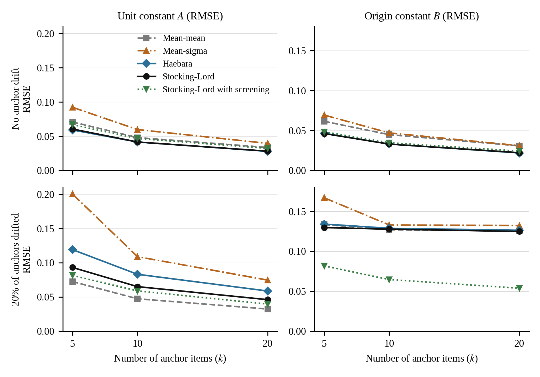
Figure 2. Root mean square error of the linking constants by method and number of anchors, without drift (upper) and with 20 per cent of anchors drifted by 0.6 on the difficulty scale (lower). 500 replications per point.

Drift changed the picture (Figure 2, lower panels; Table 3). Every unscreened method showed a bias in B of about −0.12 at all anchor lengths, which equals the drifted share of the anchors (0.20) multiplied by the drift (0.6). Adding anchors did not remove this bias, because the drifted share stayed constant. Mean-sigma was the least stable for the unit constant (RMSE of A 0.200 at k = 5), and mean-mean, which uses discriminations only for the unit, was least affected in A because the drift acted on difficulties alone. Screening reduced the bias in B to between −0.03 and −0.02 and the RMSE of the linked difficulties of the unique items from 0.173 to 0.130 at k = 10. It removed 71, 81 and 85 per cent of drifted anchors at k = 5, 10 and 20.

Table 3. Results at k = 10 anchors (500 replications). Bias and RMSE refer to constants relative to the sample-level truth; RMSE(b) refers to unique Form B items.

The cost of mechanical screening was substantial. Without drift, the rule removed at least one stable anchor in 36, 50 and 68 per cent of replications at k = 5, 10 and 20, an item-level removal rate of roughly 7 to 8 per cent, well above the 1 per cent a normal residual would suggest. Residuals of difficulty are heteroscedastic, being larger for items at the extremes of the scale, and the interquartile range is a poor scale estimate with few items. The loss of accuracy was small when anchors were stable (Figure 2), but deletion of stable items shortens the anchor and may unbalance its content, which is the concern raised in Section 5.2. Figure 3 shows one replication drawn with the first random seed, without selection. Both drifted anchors (items 5 and 10) were removed, and so was one stable anchor (item 7). On the stable anchors, the maximum characteristic-curve difference fell from 0.26 to 0.14 score units and the RMSD from 0.16 to 0.07 after screening, and the origin constant moved from 0.36 to 0.47 against a true value of 0.51.

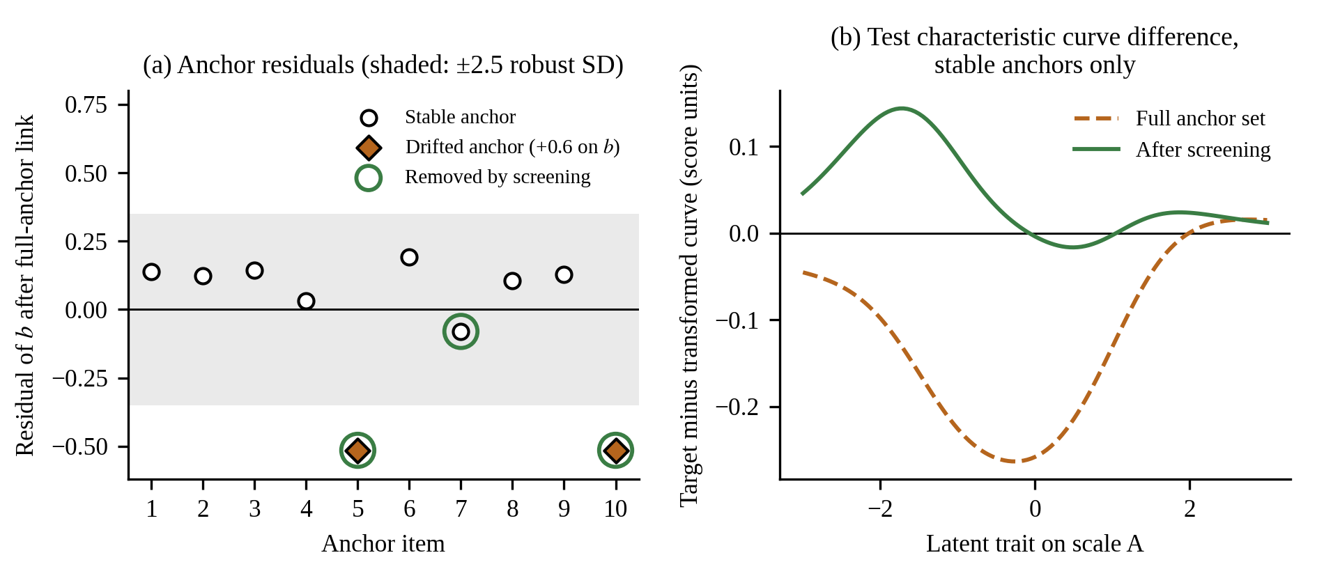
Figure 3. One illustrative replication (k = 10, two drifted anchors). (a) Residuals of anchor difficulty after Stocking-Lord linking on all anchors. (b) Difference between target and transformed test characteristic curves for the eight stable anchors, before and after screening.

Linking error was comparable to the sampling error of a group mean (Figure 4a). At k = 10 the standard deviation of the error in B was 0.037 with fixed items and 0.033 when items were redrawn, against 0.038 for the standard error of a mean of 1,000 examinees with standard deviation 1.2. Combining the two as independent sources gives a standard error about a quarter larger than the sampling error alone, so a trend or group comparison that ignored the link would understate its uncertainty by about that amount. The person bootstrap gave larger values (0.058 for A and 0.061 for B) than the sample-conditional spread. This is expected, because resampled examinees also vary in their own mean and spread, so the bootstrap estimates the total uncertainty of the group parameters on the reference scale and not the linking error alone. The effect of redrawing items was small here, because the drawn item sets were all drawn from the same broad distribution, and larger item-selection effects should be expected with heterogeneous pools.

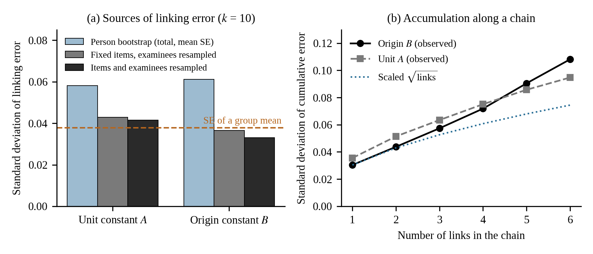
Figure 4. (a) Standard deviation of linking error in the unit and origin constants (k = 10, no drift) from three sources, with the standard error of a group mean for reference. (b) Standard deviation of the cumulative error in the constants along a chain of links.

Error accumulated along the chain (Figure 4b). The standard deviation of the cumulative error in B rose from 0.030 after one link to 0.108 after six, and that in A from 0.036 to 0.095. The growth was faster than the square-root rule that independent link errors would suggest (which gives 0.074 at six links), partly because an error in A at one link multiplies the origin constants of the earlier links. A bank maintained by repeated chained links therefore needs either a periodic re-anchoring to the reference scale or an explicit chain-error budget.

8. Recommended practice and reporting

The review and the illustration suggest a sequence for placing a new calibration on an existing metric. First, define the reference scale and record its version. Second, assemble the anchor set and screen it for content coverage, difficulty range, fit, precision, exposure and DIF or drift. Third, calibrate the new data, preferably separately, so that anchor behaviour can be inspected. Fourth, estimate the transformation with at least two defensible methods and compare them. Fifth, repeat the estimate with flagged anchors removed and record the effect. Sixth, quantify linking error, including the item-selection component where possible. Seventh, inspect curve discrepancies and plots, and only then transform the new parameters and update the bank. Eighth, record everything needed to reproduce the result. Agreement among methods, and between full and screened anchor sets, raises confidence in the link. Material disagreement should lead to investigation and not to selection of the preferred value. Table 4 lists the minimum information a linking report should contain.

Table 4. Minimum reporting standard for an IRT linking study.

9. Implications for PsychtrixWeb

For an online psychometric platform the main consequence is that linking should be managed as a record and not only as a calculation. Six design features follow from the review. Every linking operation should display its source metric, target metric and transformation equation, since constants without direction invite misuse. A scale registry should hold versioned metrics, each with an identifier and status, together with the documented transformation between successive versions, so that scores can be reproduced years later. An anchor registry should store for each item its linking occasions, groups, DIF and drift history, exposure and current eligibility. The linking module should offer more than one method and show their constants side by side with curve discrepancies and bootstrap uncertainty, so that sensitivity is visible at the point of decision, and automatic anchor flags should assist expert judgement and not replace it, for the reasons shown in Section 7. A linking graph should show how each form connects to the reference scale, the length of every chain and any isolated form. Finally, the internal IRT metric should be kept separate from the reporting metric, for example T = 50 + 10θ, so that reporting conventions can change without recalibration. An audit trail recording analyst, date, anchor exclusions and approval status, and a periodic audit of drift, DIF, exposure and constants, complete the design. These are proposals for software design and have not yet been evaluated with users.

10. Limitations

The review is selective and not systematic. The simulation used a correctly specified unidimensional 2PL model, drift acting on difficulty only and in one direction, one sample size, one pattern of item parameters and one screening rule, and the symmetric criteria and weights were implementation choices. Models with misfit, guessing, polytomous items or multidimensionality may behave differently. The sample-level definition of truth isolates linking error from person sampling but is not the only reasonable definition. No empirical dataset was analysed, and the platform architecture is a proposal. The qualitative conclusions, that characteristic-curve methods are more accurate with stable anchors, that drift biases the origin constant in proportion to its share, that mechanical screening has a price, and that linking error is not negligible for aggregates, agree with the studies cited, but the numerical values apply only to the conditions simulated.

11. Conclusion

Calibration produces item parameters, but it does not by itself make them comparable across datasets. Because the latent metric is fixed only by constraints applied within each calibration, separately calibrated parameters need a linking procedure before they can be read on one scale. Shared items, shared persons or randomised groups supply the connection, and the quality of the result depends on the anchors, the model, the calibration and the stability of the linking items. Characteristic-curve methods generally use the anchor information better than moment methods, but no method protects against unstable anchors, and mechanical deletion of items is a poor substitute for judgement. The uncertainty of the link should be reported, particularly for aggregate comparisons and for chains, where it accumulates.

Linking, equating and invariance remain different questions. A successful link establishes a metric. It does not equate forms, and it does not show that the construct functions in the same way across groups or occasions. For an evolving item bank the practical requirement is a documented measurement metric, with its calibration history, anchor history, transformations, drift and DIF evidence, and uncertainty. The next question in this series is how that metric is maintained under changing populations and repeated measurement.

Data and code availability. The study used simulated data only. The Python code that generated all results and figures is supplied with this note.

References

- Baker, F. B. (1992). Equating tests under the graded response model. Applied Psychological Measurement, 16(1), 87-96.
- Battauz, M. (2013). IRT test equating in complex linkage plans. Psychometrika, 78(3), 464-480. https://doi.org/10.1007/s11336-012-9316-y
- Battauz, M. (2017). Multiple equating of separate IRT calibrations. Psychometrika, 82(3), 610-636. https://doi.org/10.1007/s11336-016-9517-x
- Bock, R. D., & Zimowski, M. F. (1997). Multiple group IRT. In W. J. van der Linden & R. K. Hambleton (Eds.), Handbook of modern item response theory (pp. 433-448). Springer.
- Bock, R. D., Muraki, E., & Pfeiffenberger, W. (1988). Item pool maintenance in the presence of item parameter drift. Journal of Educational Measurement, 25(4), 275-285.
- Candell, G. L., & Drasgow, F. (1988). An iterative procedure for linking metrics and assessing item bias in item response theory. Applied Psychological Measurement, 12(3), 253-260. https://doi.org/10.1177/014662168801200304
- Choi, S. W., Schalet, B., Cook, K. F., & Cella, D. (2014). Establishing a common metric for depressive symptoms: Linking the BDI-II, CES-D, and PHQ-9 to PROMIS Depression. Psychological Assessment, 26(2), 513-527.
- Donoghue, J. R., & Isham, S. P. (1998). A comparison of procedures to detect item parameter drift. Applied Psychological Measurement, 22(1), 33-51.
- Embretson, S. E., & Reise, S. P. (2000). Item response theory for psychologists. Lawrence Erlbaum.
- Fischer, L., Rohm, T., Carstensen, C. H., & Gnambs, T. (2021). Linking of Rasch-scaled tests: Consequences of limited item pools and model misfit. Frontiers in Psychology, 12, Article 633896. https://doi.org/10.3389/fpsyg.2021.633896
- Haberman, S. J. (2009). Linking parameter estimates derived from an item response model through separate calibrations (ETS Research Report No. RR-09-40). Educational Testing Service. https://doi.org/10.1002/j.2333-8504.2009.tb02197.x
- Haebara, T. (1980). Equating logistic ability scales by a weighted least squares method. Japanese Psychological Research, 22(3), 144-149.
- Hanson, B. A., & Béguin, A. A. (2002). Obtaining a common scale for item response theory item parameters using separate versus concurrent estimation in the common-item equating design. Applied Psychological Measurement, 26(1), 3-24.
- Holland, P. W., & Dorans, N. J. (2006). Linking and equating. In R. L. Brennan (Ed.), Educational measurement (4th ed., pp. 187-220). American Council on Education and Praeger.
- Hu, H., Rogers, W. T., & Vukmirovic, Z. (2008). Investigation of IRT-based equating methods in the presence of outlier common items. Applied Psychological Measurement, 32(4), 311-333. https://doi.org/10.1177/0146621606292215
- Kim, S. (2006). A comparative study of IRT fixed parameter calibration methods. Journal of Educational Measurement, 43(4), 355-381.
- Kim, S.-H., & Cohen, A. S. (1998). A comparison of linking and concurrent calibration under item response theory. Applied Psychological Measurement, 22(2), 131-143.
- Klein, L. W., & Jarjoura, D. (1985). The importance of content representation for common-item equating with nonrandom groups. Journal of Educational Measurement, 22(3), 197-206.
- Kolen, M. J., & Brennan, R. L. (2014). Test equating, scaling, and linking: Methods and practices (3rd ed.). Springer.
- Kopf, J., Zeileis, A., & Strobl, C. (2015). Anchor selection strategies for DIF analysis: Review, assessment, and new approaches. Educational and Psychological Measurement, 75(1), 22-56. https://doi.org/10.1177/0013164414529792
- Li, Y. (2012). Examining the impact of drifted polytomous anchor items on test characteristic curve (TCC) linking and IRT true score equating (ETS Research Report No. RR-12-09). Educational Testing Service.
- Lord, F. M. (1980). Applications of item response theory to practical testing problems. Lawrence Erlbaum.
- Loyd, B. H., & Hoover, H. D. (1980). Vertical equating using the Rasch model. Journal of Educational Measurement, 17(3), 179-193.
- Marco, G. L. (1977). Item characteristic curve solutions to three intractable testing problems. Journal of Educational Measurement, 14(2), 139-160.
- Masters, G. N. (1982). A Rasch model for partial credit scoring. Psychometrika, 47(2), 149-174.
- Meredith, W. (1993). Measurement invariance, factor analysis and factorial invariance. Psychometrika, 58(4), 525-543.
- Michaelides, M. P. (2010). A review of the effects on IRT item parameter estimates with a focus on misbehaving common items in test equating. Frontiers in Psychology, 1, Article 167. https://doi.org/10.3389/fpsyg.2010.00167
- Michaelides, M. P., & Haertel, E. H. (2014). Selection of common items as an unrecognized source of variability in test equating: A bootstrap approximation assuming random sampling of common items. Applied Measurement in Education, 27(1), 46-57.
- Millsap, R. E. (2011). Statistical approaches to measurement invariance. Routledge.
- Monseur, C., & Berezner, A. (2007). The computation of equating errors in international surveys in education. Journal of Applied Measurement, 8(3), 323-335.
- Muraki, E. (1992). A generalized partial credit model: Application of an EM algorithm. Applied Psychological Measurement, 16(2), 159-176.
- Ogasawara, H. (2001). Standard errors of item response theory equating/linking by response function methods. Applied Psychological Measurement, 25(1), 53-67.
- Oladunmoye E.O (2025). Ultra-short scales in employee assessment: balancing efficiency and accuracy. Journal of Applied Sciences, Information and Computing.6(2),103-108.
- Oladunmoye, E. O. (2026a). The Rasch model and 1PL IRT: Understanding item difficulty, person ability, and invariant measurement. PsychtrixWeb Research Notes, 012.
- Oladunmoye, E. O. (2026b). The two-parameter logistic IRT model: Understanding item discrimination, difficulty, and differential item functioning. PsychtrixWeb Research Notes, 013.
- Oladunmoye, E. O. (2026c). Validity in psychological measurement: Beyond reliability and statistical significance. PsychtrixWeb Research Notes, 003.
- Oladunmoye, E. O., (2015). Development and validation of social provision scale on first year undergraduate psychological adjustment. Journal of Education and Practice, 6 (28), 78-90.
- Oladunmoye, E. O., Muhammad T. S., (2024). Development and Validation of Multiple Intelligence Test among emerging adults in the United Kingdom. ISAR Journal of Arts, Humanities and Social Sciences, 2(4), 18-24.
- Oladunmoye, E.O., Agbor, E.C., Olabisi, O.L., and Oyadeyi, J.B., (2024). Estimating measurement invariance on emotional intelligence scale across gender and age among undergraduates in Nigeria. Thinking Skills and Creativity Journal. 7(1),50-60
- Oladunmoye, E.O., Enamudu, G.P., Ogbu, F. (2024). Comparison of estimate of linear and Equi-percentile CTT equating of WAEC Mathematics test forms 2022 and 2023. International Journal of Humanities Social Science and Management (IJHSSM), 4(3),544-552.
- Oladunmoye, E.O., Enamudu, G.P., Sa'ad, M.T. (2024). A Differential Item Functioning estimate of WAEC Mathematics test form based on gender and age among secondary school students. ISAR Journal of Multidisciplinary Research and Studies, 2(5), 15-21.
- Oshima, T. C., Davey, T. C., & Lee, K. (2000). Multidimensional linking: Four practical approaches. Journal of Educational Measurement, 37(4), 357-373.
- Putnick, D. L., & Bornstein, M. H. (2016). Measurement invariance conventions and reporting: The state of the art and future directions for psychological research. Developmental Review, 41, 71-90.
- Reckase, M. D. (2009). Multidimensional item response theory. Springer.
- Reeve, B. B., Hays, R. D., Bjorner, J. B., Cook, K. F., Crane, P. K., Teresi, J. A., Thissen, D., Revicki, D. A., Weiss, D. J., Hambleton, R. K., Liu, H., Gershon, R., Reise, S. P., Lai, J. S., & Cella, D. (2007). Psychometric evaluation and calibration of health-related quality of life item banks: Plans for the Patient-Reported Outcomes Measurement Information System (PROMIS). Medical Care, 45(5, Suppl. 1), S22-S31.
- Samejima, F. (1969). Estimation of latent ability using a response pattern of graded scores. Psychometrika Monograph Supplement, 34(4, Pt. 2), No. 17.
- Sheehan, K. M., & Mislevy, R. J. (1988). Some consequences of the uncertainty in IRT linking procedures (ETS Research Report No. RR-88-38-ONR). Educational Testing Service. https://doi.org/10.1002/j.2330-8516.1988.tb00294.x
- Sinharay, S., & Holland, P. W. (2010). The missing data assumptions of the NEAT design and their implications for test equating. Psychometrika, 75(2), 309-327.
- Stocking, M. L., & Lord, F. M. (1983). Developing a common metric in item response theory. Applied Psychological Measurement, 7(2), 201-210. https://doi.org/10.1177/014662168300700208
- Tong, Y., & Kolen, M. J. (2007). Comparisons of methodologies and results in vertical scaling for educational achievement tests. Applied Measurement in Education, 20(2), 227-253.
- van de Vijver, F., & Leung, K. (1997). Methods and data analysis for cross-cultural research. Sage.
- van der Linden, W. J., & Barrett, M. D. (2016). Linking item response model parameters. Psychometrika, 81(3), 650-673. https://doi.org/10.1007/s11336-015-9469-6
- van der Linden, W. J., & Glas, C. A. W. (Eds.). (2010). Elements of adaptive testing. Springer.
- von Davier, M., & von Davier, A. A. (2007). A unified approach to IRT scale linking and scale transformation. Methodology, 3(3), 115-124. (Original work published 2004 as ETS Research Report No. RR-04-09)
- Wainer, H., Dorans, N. J., Eignor, D., Flaugher, R., Green, B. F., Mislevy, R. J., Steinberg, L., & Thissen, D. (2000). Computerized adaptive testing: A primer (2nd ed.). Lawrence Erlbaum.
- Wingersky, M. S., Cook, L. L., & Eignor, D. R. (1987). Specifying the characteristics of linking items used for item response theory item calibration (ETS Research Report No. RR-87-24). Educational Testing Service.
- Wu, M. (2010). Measurement, sampling, and equating errors in large-scale assessments. Educational Measurement: Issues and Practice, 29(4), 15-27.
Suggested citation
Oladunmoye, E. O. (2026). Item Response Theory Calibration and Linking: Establishing a Common Measurement Scale Across Samples, Forms and Time. PsychtrixWeb Research Note, 019. Psychtrix Initiative Limited. https://doi.org/10.5281/zenodo.23307668Discuss this Research Note
Scholarly comments are welcome from anyone — no account required. Contributions are moderated before they appear.
No comments yet. Start the scholarly discussion below.