Interpreting Item Characteristic Curves in Item Response Theory: A Practical and Methodological Guide

1. Introduction 

Item response theory (IRT) represents a substantial departure from the logic of classical test theory. Rather than treating the total observed score as the primary unit of analysis, IRT models the probability of a particular response as a joint function of a respondent's position on a latent trait and the measurement properties of the item itself (Hambleton, Swaminathan & Rogers, 1991; Embretson & Reise, 2000). The item characteristic curve is the most intuitive graphical expression of this idea: it converts an abstract set of item parameters into a visible curve that describes how the probability of a response changes as the latent trait increases.

This intuitive appeal is also a source of risk. An ICC can be produced automatically by almost any modern IRT program, researchers sometimes evaluate it superficially, judging a curve as "good" simply because it forms a recognisable S-shape, without examining its location, slope, asymptotic behaviour, range of effective measurement, or relationship to item information and model fit. This note builds on earlier notes in this series that introduced the general logic of latent-trait measurement and the one-, two-, three- and four-parameter logistic models (Oladunmoye, 2026a, 2026b, 2026c, 2026d, 2026e), and asks a more practical question: how should a researcher actually interpret an ICC in a way that is defensible, reproducible and useful for decision-making about items and tests?

The remainder of the note proceeds as follows. Section 2 defines the ICC formally and explains why it should be treated as a model-implied function rather than a descriptive plot of raw data. Section 3 reviews how item location, discrimination and the lower and upper asymptotes shape the curve under the 1PL, 2PL, 3PL and 4PL models. Section 4 proposes a structured interpretation framework built around four guiding questions and illustrates it with a worked example. Section 5 relates the ICC to the item information function, the test characteristic curve, the test information function and differential item functioning. Section 6 sets out methodological standards, including common misinterpretations and their corrections, and Section 7 applies the framework to a small simulated item bank. Section 8 briefly considers the implications for psychometric software, and Section 9 concludes.

2. Conceptual Definition of the Item Characteristic Curve

For a dichotomously scored item, the ICC represents the conditional probability of a positive or correct response given the latent trait:

P_i(X_i = 1 | θ) = P(θ)

where Xi = 1 denotes a positive or correct response, θ (theta) represents the latent trait, and P denotes the model-implied probability of that response. Conventionally the horizontal axis represents θ, typically standardised to a mean of zero and a standard deviation of one, and the vertical axis represents the probability of the specified response, ranging from 0 to 1. A value of 0.80 at a given θ therefore means that the fitted model implies an 80 per cent probability of the specified response at that level of the trait, not that 80 per cent of respondents at that trait level actually gave that response in the observed sample.

2.1 The ICC as a model-implied function

This last distinction is central to sound interpretation. An ICC is not a smoothed scatterplot of raw item scores against an observed score; it is generated from an estimated statistical model (Lord, 1980; Birnbaum, 1968). Consequently, an ICC should never be interpreted in isolation from the assumptions on which it rests: the choice of model, the precision of the parameter estimates, the fit of the model to the data, the dimensionality of the item set, the assumption of local independence, and the characteristics of the calibration sample (American Educational Research Association, American Psychological Association and National Council on Measurement in Education [AERA, APA & NCME], 2014). A visually attractive, well-behaved S-shaped curve can still belong to a model that fits the data poorly, so a curve's appearance is a starting point for enquiry rather than a conclusion in itself.

3. Item Response Models and the Shape of the ICC

The exact form of the ICC depends on the IRT model chosen. This section summarises the one- and two-parameter logistic models, in which location and discrimination are the operative parameters, and the three- and four-parameter models, which additionally allow for a non-zero lower asymptote and a sub-unity upper asymptote.

3.1 Location and discrimination in the 1PL and 2PL models

Under the two-parameter logistic (2PL) model, the probability of a positive response is given by:

P_i(θ) = 1 / {1 + exp[-a_i(θ - b_i)]}

The parameter ai is the discrimination parameter and bi is the location, or difficulty, parameter. The 2PL therefore tells the researcher two fundamental things about an item: where along the trait continuum it operates, and how sharply it differentiates respondents around that point. Setting ai to a common value across items recovers the one-parameter logistic (1PL, or Rasch) model, in which only location varies. Figure 1 illustrates both effects. In panel (a), three curves share a common discrimination but differ in location: a curve shifted to the left indicates that the item is answered correctly, or endorsed, at comparatively lower levels of the trait, while a curve shifted to the right indicates that higher trait levels are required. In panel (b), three curves share a common location but differ in discrimination: a steeper curve reflects stronger local differentiation among respondents near that location, whereas a flatter curve indicates that changes in θ produce comparatively small changes in response probability.

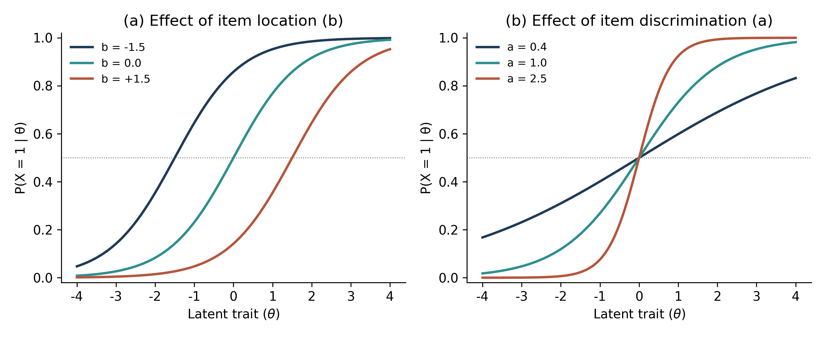
Figure 1. Item characteristic curves illustrating (a) the effect of item location (b) holding discrimination constant at a = 1.2, and (b) the effect of discrimination (a) holding location constant at b = 0. Curves were generated from the two-parameter logistic model.

Two qualifications are worth stating explicitly, because they are frequently misunderstood in applied reports. First, the difference between two location parameters, for example b = 2.0 and b = 1.0, represents a one-unit separation on the latent metric; it is not a ratio, and an item with b = 2.0 is not "twice as difficult" as one with b = 1.0. Second, a steep curve indicates strong local discrimination, but discrimination is not, by itself, a global indicator of item quality: an item with very high a may function well only across a narrow region of the trait, may show local dependence with other items, may behave differently across subgroups, or may otherwise be well estimated but substantively weak. Discrimination should therefore be read alongside content evidence, model fit and fairness analysis rather than used as a stand-alone selection criterion.

3.2 Lower and upper asymptotes in the 3PL and 4PL models

The three-parameter logistic (3PL) model introduces a lower asymptote, ci, which allows the curve to approach a non-zero probability at very low values of θ:

P_i(θ) = c_i + (1 - c_i) / {1 + exp[-a_i(θ - b_i)]}

In a multiple-choice context this lower asymptote is sometimes associated with pseudo-guessing behaviour, but ci is a model parameter describing lower-tail response probability, and it should not be treated as a direct behavioural measurement of guessing at the level of the individual respondent (Loken and Rulison, 2010). The four-parameter logistic (4PL) model adds a further parameter, di, representing an upper asymptote below one:

P_i(θ) = c_i + (d_i - c_i) / {1 + exp[-a_i(θ - b_i)]}

A value of di below one implies that even very high-trait respondents are not modelled as certain to respond correctly, an allowance sometimes associated with careless responding, fatigue or slipping (Waller and Reise, 2010). As with the lower asymptote, the quantity 1 - di is a model-implied ceiling and should not, on its own, be read as an individual-level index of carelessness. Figure 2 illustrates both extensions.

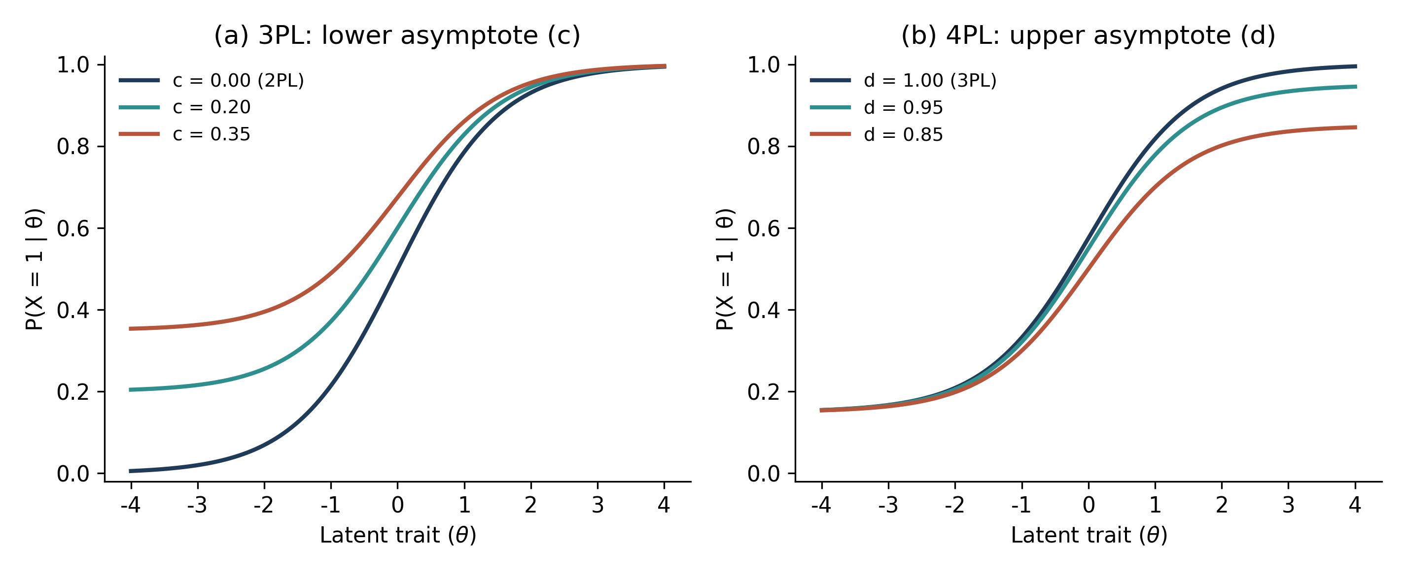
Figure 2. (a) Three-parameter logistic curves with a common location and discrimination but varying lower asymptote (c). (b) Four-parameter logistic curves with a common location, discrimination and lower asymptote but varying upper asymptote (d).

The logic of the ICC extends, with some adaptation, to polytomous items. In models such as Samejima's (1969) graded response model, each response category has its own category response curve describing the probability of selecting that category as a function of θ. Researchers working with ordered response formats, common in psychological scales using Likert-type items, should inspect whether categories are ordered and clearly differentiated across the trait continuum; extensive overlap among category curves can indicate that respondents are not reliably distinguishing between adjacent response options, which is a useful diagnostic in its own right and is not visible from category frequencies alone.

4. A Structured Interpretation Framework

A practical starting point for ICC interpretation is a small set of guiding questions, summarised in Table 1. These questions correspond directly to the parameters introduced in Section 3 and provide a consistent vocabulary for describing an item, whichever software or reporting template is used.

Table 1. Four guiding questions for a structured reading of an item characteristic curve.

4.1 Worked example: comparing item location at constant discrimination

Numerical parameter tables can obscure differences that are immediately visible once curves are plotted. Table 2 lists three simulated items sharing an identical discrimination parameter but differing in location.

Table 2. Three simulated items with identical discrimination but differing location parameters.

Because the three items share a common discrimination, the parameter table alone might suggest that they are functionally interchangeable. Plotting the corresponding ICCs, as in Figure 1(a), shows immediately that the items are shifted horizontally and therefore serve different measurement purposes: item A is best suited to distinguishing respondents at the lower end of the trait, item C at the upper end, and item B near the centre of the distribution. A parameter table combined with graphical inspection is consistently more informative than either source considered alone.

4.2 Item targeting and test-level design

The same logic extends from single items to a test as a whole. A well-targeted test contains items whose locations span the region of the trait continuum where measurement precision is actually required. If the respondent sample lies predominantly between θ = -1.5 and θ = +1.5, but the item pool is dominated by items with b values above 2.5, the curves for those items will be concentrated too far to the right of the region in which most respondents are located, and measurement precision will suffer where it matters most. This is one reason that item selection should be informed by the intended use of the test and the expected distribution of the target population, not by a discrimination threshold applied in isolation.

5. Relating the ICC to Other Psychometric Functions

The ICC is one of several complementary functions used in IRT-based item evaluation, and it answers a narrower question than researchers sometimes assume: it describes the probability of a response at each level of the trait, not the precision with which the item measures that trait, nor how a group of items functions collectively.

5.1 The item information function

The item information function (IIF) indicates the levels of θ at which a given item measures most precisely. For the general logistic form used here, information can be expressed as:

I_i(θ) = a_i²[P_i(θ) - c_i]²[d_i - P_i(θ)]² / {(d_i - c_i)²P_i(θ)[1 - P_i(θ)]}

which reduces to the familiar Ii(θ) = ai²Pi(θ)[1 - Pi(θ)] under the 2PL, where ci = 0 and di = 1. An item may be highly informative near θ = 0 while contributing very little information near θ = 2.5, so a statement such as "this item is reliable" is incomplete without reference to the region of the trait continuum to which it applies. Figure 3 places the ICC and the IIF for a single simulated item side by side, illustrating that item information peaks near the item's location and falls away towards the extremes of the trait continuum, most sharply for items with high discrimination and non-trivial asymptotes.

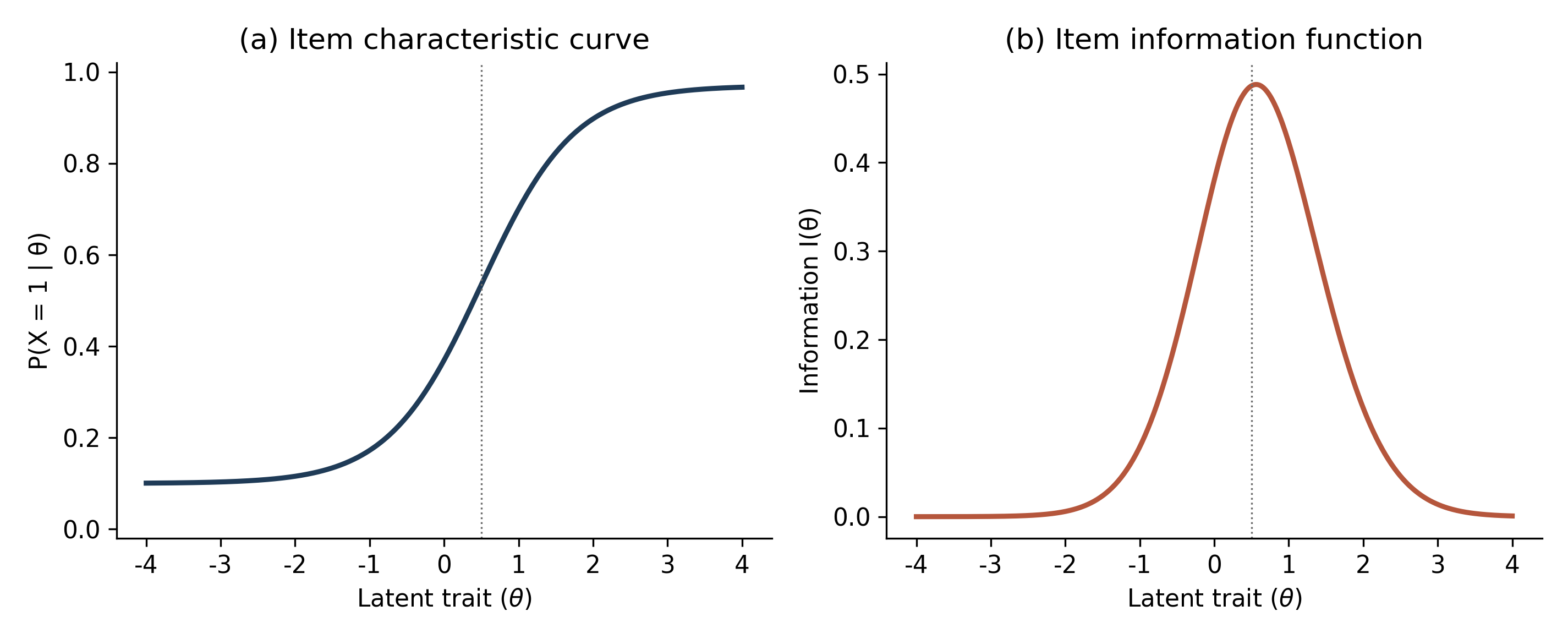
Figure 3. (a) Item characteristic curve and (b) corresponding item information function for a simulated four-parameter item (a = 1.6, b = 0.5, c = 0.10, d = 0.97). The dotted line marks the item's location, near which information is greatest.

5.2 The test characteristic curve and test information function

At the test level, the test characteristic curve (TCC) gives the expected observed score as a function of θ, obtained by summing the individual ICCs of the items that make up the test:

TCC(θ) = Σ P_i(θ), for i = 1 to k

The test information function is obtained analogously by summing the item information functions, Itest(θ) = ΣIi(θ), and indicates where the test as a whole provides the greatest measurement precision. The design objective is rarely to maximise information everywhere; rather, it is to concentrate precision where measurement is substantively required, whether that is around a diagnostic threshold, a policy cut score, or the centre of the population distribution. Figure 4 shows the TCC and test information function for a simulated six-item pool with locations spread across the trait continuum.

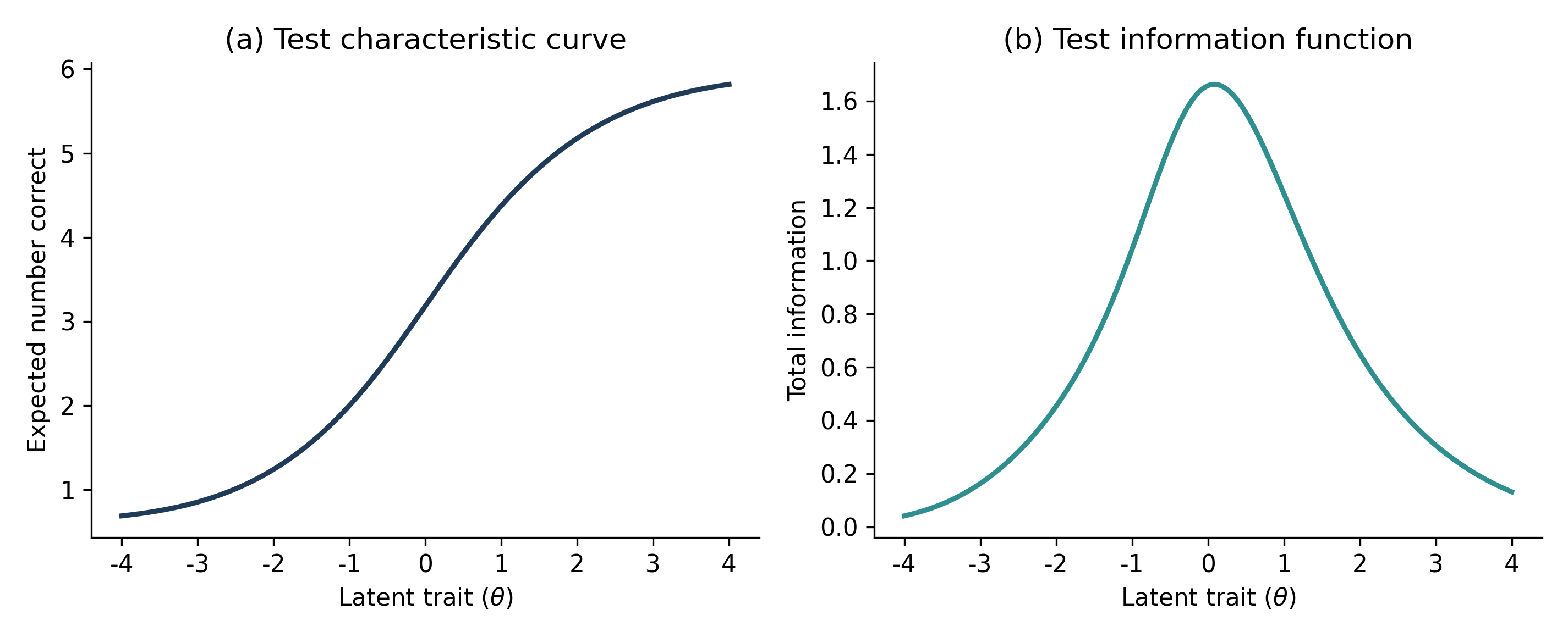
Figure 4. (a) Test characteristic curve and (b) test information function for a simulated six-item pool with locations spanning theta = -1.8 to +2.0.

5.3 ICCs and differential item functioning

ICCs are also a natural way to visualise differential item functioning (DIF), the phenomenon in which an item's response function differs across groups after conditioning on the latent trait (Oladunmoye, Enamudu, & Sa'ad, 2024; Holland & Wainer, 1993). When curves for a reference and a focal group are approximately parallel but horizontally offset, the pattern is typically described as uniform DIF, indicating a difference in location between groups. When the curves differ in slope, and consequently cross at some point along the trait continuum, the pattern is described as non-uniform DIF. With 3PL or 4PL models, group differences may also appear in the lower or upper asymptotes. Figure 5 illustrates both uniform and non-uniform patterns using simulated reference and focal group curves.

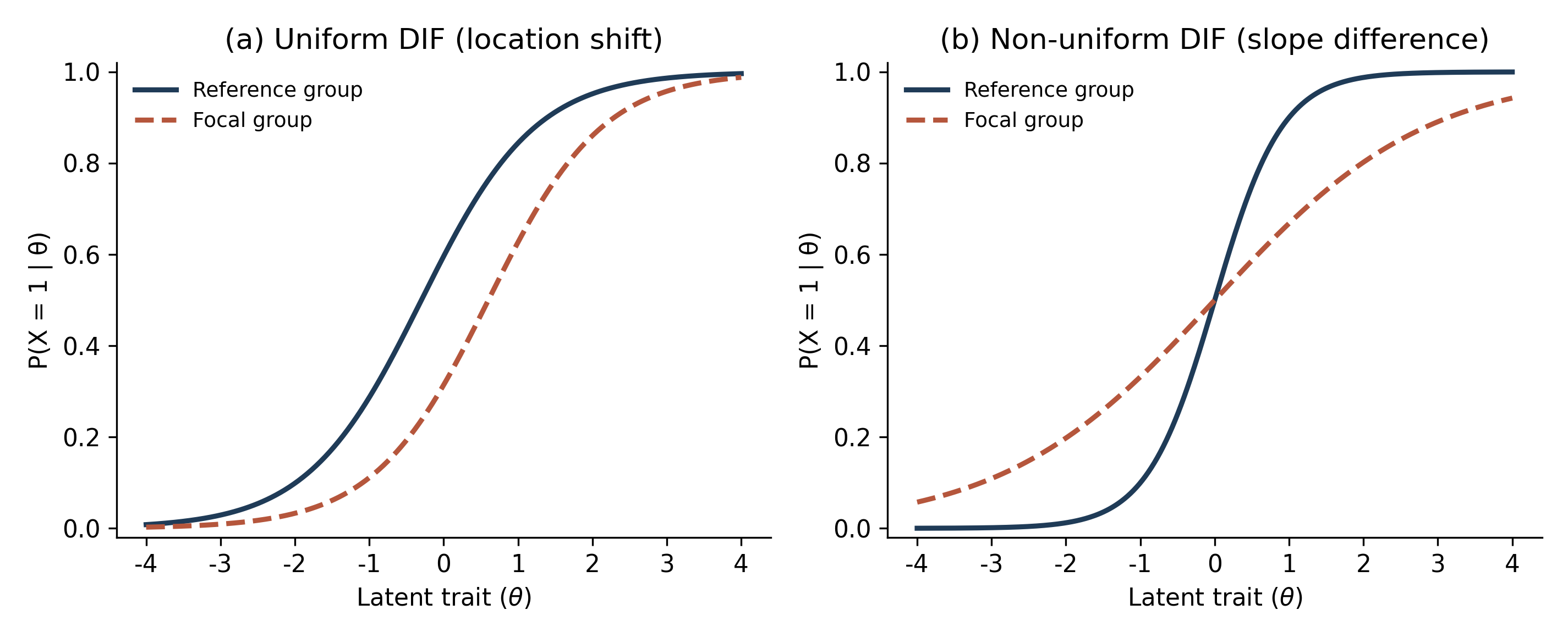
Figure 5. Simulated differential item functioning. (a) Uniform DIF, in which the focal group curve is shifted to a higher location than the reference group curve. (b) Non-uniform DIF, in which the two groups differ in discrimination and the curves cross.

6. Methodological Standards for ICC-Based Item Evaluation

6.1 The limits of visual inspection

A curve should never be judged by appearance alone. Whether the empirical response data are adequately represented by the fitted model should be assessed with formal diagnostics, including item-fit statistics such as the S-X² index (Orlando & Thissen, 2000), residual analyses comparing observed and model-expected response proportions across intervals of the trait continuum, checks for local dependence among items, and, at the model level, comparative fit indices. A model can generate a visually plausible, well-formed curve while nonetheless departing from the empirical data in ways that only these diagnostics will reveal, so visual inspection is a necessary complement to, but not a substitute for, formal fit assessment (AERA, APA & NCME, 2014).

A further precondition for meaningful interpretation concerns the direction of scoring. Before an ICC is interpreted substantively, the researcher should establish what higher θ represents for the construct in question, for example greater depressive symptom severity on a clinical scale or greater self-efficacy on a confidence measure, and what a response coded as X = 1 represents for the item concerned. Reverse-keyed items are a common source of error here: if agreement with an item such as "I feel unable to cope with everyday problems" indicates poorer wellbeing, the raw response direction may run counter to the intended orientation of the latent trait, and the ICC cannot itself correct for incorrect scoring. These checks belong in data preparation, before IRT calibration, rather than at the interpretation stage.

6.2 Common misinterpretations and their corrections

Several recurring errors appear in applied reports that rely on ICCs. Table 3 summarises the most frequent of these alongside the corresponding correction.

Table 3. Frequent misinterpretations of item characteristic curves and the corresponding methodological correction.

6.3 Reporting standards for publication

A publication-quality ICC figure should include clearly labelled axes, a stated theta range appropriate to the sample and purpose, an item identifier, the fitted model specification, a legend where more than one curve is shown, and a caption that states how the curve was estimated. In text, descriptive language should specify both the direction and the conditional nature of any probability statement. A sentence such as "the item characteristic curves indicated substantial variation in item location and discrimination, with higher-discrimination items showing steeper response functions around their respective locations" conveys considerably more than the unqualified assertion that "the ICCs were good", and it gives the reader enough information to evaluate the claim independently.

7. A Worked Illustration: Item-Level Reporting in Practice

Table 4 presents a simulated item-level summary of the kind that a psychometric analysis platform might generate once a model has been fitted. The intention is to show how the numerical parameters, the ICC, and diagnostic information are typically brought together in a single record for reporting and item-bank management.

Table 4. Simulated item-level summary combining parameter estimates with fit and fairness diagnostics.

A structured narrative summary of this item might read: this item demonstrates moderate-to-high discrimination and is targeted towards respondents with above-average trait levels; the curve shows a lower asymptote of approximately 0.12 and an upper asymptote of approximately 0.95; the S-X² statistic gives no indication of misfit, and no DIF was detected across the grouping variable examined. Such a summary deliberately stops short of an unqualified verdict such as "this item is good", because that judgement depends on additional considerations, including content coverage, the purpose of the test and the population in which it will be used.

The corresponding workflow can be summarised as a short sequence: specify the model, estimate parameters, generate the ICC, inspect a, b, c and d, evaluate item information, evaluate item fit, evaluate DIF, review item content, and only then decide whether to retain, revise or further investigate the item. This sequence is more defensible than item selection based on a single discrimination threshold, because it requires each item to clear several independent forms of evidence before being retained.

8. Implications for Psychometric Software

The workflow described above has direct implications for the design of IRT analysis software. At minimum, a usable ICC module should allow generation and inspection of curves under the 1PL, 2PL, 3PL and 4PL models, together with confidence bands, comparison of empirical and model-implied curves, side-by-side comparison of multiple items, and group-specific curves for DIF screening. It should present item information, test information and item-fit statistics alongside the ICC rather than as separate, disconnected outputs, and it should record sufficient metadata, including model specification, estimation method, sample size, and software version, to support reproducible analysis (Chalmers, 2012; de Ayala, 2022). Platforms such as PsychtrixWeb are well placed to implement this kind of integrated reporting, moving ICC generation from a simple graphing utility towards a decision-support tool that helps researchers interpret, compare and report items rather than merely plot them.

9. Conclusion

The item characteristic curve is a powerful interpretive device because it translates abstract item parameters into a visible account of how response probability changes across the latent trait. For the 1PL and 2PL models, the curve chiefly communicates location and discrimination; for the 3PL, the lower asymptote becomes relevant; and for the 4PL, the upper asymptote is added (Oladunmoye, 2026d). None of this information, however, should be interpreted in isolation. A defensible reading of an ICC integrates the curve with item information, test information, model fit, differential item functioning and content evidence, and stops short of treating any single element, including the curve's shape, as sufficient grounds for a verdict on item quality.

For applied researchers, the practical implication is straightforward: an ICC should be read as a claim about a fitted model, not as a self-evident picture of an item's worth. Reporting that specifies the trait range, the model used, and the diagnostics consulted allows readers to evaluate that claim for themselves, which is the basis of transparent and reproducible psychometric practice.

Key recommendations

• Report the fitted model, the theta range and the estimation method whenever an ICC is presented.
• Interpret location and discrimination as relative, interval-scale quantities, not as ratio statements about difficulty.
• Treat lower and upper asymptotes as model parameters, not as direct behavioural measures of guessing or carelessness.
• Pair every ICC with its item information function, and consider test-level information alongside individual items.
• Use group-specific ICCs to screen for uniform and non-uniform DIF before finalising an item bank.
• Confirm model fit with formal statistics such as S-X², since a plausible curve shape does not itself establish fit.
• Check scoring direction and reverse-keyed items before calibration, since an ICC cannot correct incorrect coding.
• Base item retention decisions on the combination of discrimination, targeting, fit, fairness and content evidence, not on any one criterion alone.

Suggested citation

Oladunmoye, E. O. (2026). Interpreting item characteristic curves in item response theory: A practical and methodological guide. PsychtrixWeb Research Notes, 015. Psychtrix Initiative Limited.

References

- American Educational Research Association, American Psychological Association, and National Council on Measurement in Education. (2014). Standards for educational and psychological testing. American Educational Research Association.
- Baker, F. B. (2001). The basics of item response theory (2nd ed.). ERIC Clearinghouse on Assessment and Evaluation.
- Baker, F. B., and Kim, S.-H. (2004). Item response theory: Parameter estimation techniques (2nd ed.). CRC Press.
- Birnbaum, A. (1968). Some latent trait models and their use in inferring an examinee's ability. In F. M. Lord and M. R. Novick (Eds.), Statistical theories of mental test scores (pp. 397 to 479). Addison-Wesley.
- Chalmers, R. P. (2012). mirt: A multidimensional item response theory package for the R environment. Journal of Statistical Software, 48(6), 1 to 29.
- de Ayala, R. J. (2022). The theory and practice of item response theory (2nd ed.). Guilford Press.
- Embretson, S. E., and Reise, S. P. (2000). Item response theory for psychologists. Lawrence Erlbaum Associates.
- Hambleton, R. K., Swaminathan, H., and Rogers, H. J. (1991). Fundamentals of item response theory. Sage Publications.
- Holland, P. W., and Wainer, H. (Eds.). (1993). Differential item functioning. Lawrence Erlbaum Associates.
- Loken, E., and Rulison, K. L. (2010). Estimation of a four-parameter item response theory model. British Journal of Mathematical and Statistical Psychology, 63(3), 509 to 525.
- Lord, F. M. (1977). Practical applications of item characteristic curve theory. Journal of Educational Measurement, 14(2), 117 to 138.
- Lord, F. M. (1980). Applications of item response theory to practical testing problems. Lawrence Erlbaum Associates.
- Oladunmoye, E. O. (2026a). Item response theory: From observed responses to latent trait measurement. PsychtrixWeb Research Notes, 011.
- Oladunmoye, E. O. (2026b). The Rasch model and 1PL IRT: Understanding item difficulty, person ability and invariant measurement. PsychtrixWeb Research Notes, 012.
- Oladunmoye, E. O. (2026c). The two-parameter logistic IRT model: Understanding item discrimination, difficulty and differential item functioning. PsychtrixWeb Research Notes, 013.
- Oladunmoye, E. O. (2026d). The 3PL and 4PL item response theory models: Modelling guessing, slipping and upper-asymptote behaviour. PsychtrixWeb Research Notes, 014.
- Oladunmoye, E. O. (2026e). Understanding Psychometric Measurement. PsychtrixWeb Research Note, 003. Psychtrix Initiative Limited. https://doi.org/10.5281/zenodo.22653162.
- Oladunmoye, E.O., Enamudu, G.P., Sa'ad, M.T. (2024). A Differential Item Functioning estimate of WAEC Mathematics test form based on gender and age among secondary school students. ISAR Journal of Multidisciplinary Research and Studies, 2(5), 15-21.
- Orlando, M., and Thissen, D. (2000). Likelihood-based item-fit indices for dichotomous item response theory models. Applied Psychological Measurement, 24(1), 50 to 64.
- Rasch, G. (1960). Probabilistic models for some intelligence and attainment tests. Danish Institute for Educational Research.
- Reise, S. P., and Waller, N. G. (2009). Item response theory and clinical measurement. Annual Review of Clinical Psychology, 5, 27 to 48.
- Samejima, F. (1969). Estimation of latent ability using a response pattern of graded scores. Psychometrika Monograph, No. 17.
- Waller, N. G., and Reise, S. P. (2010). Measuring psychopathology with nonstandard item response theory models: Fitting the four-parameter model to the MMPI. In S. E. Embretson (Ed.), Measuring psychological constructs: Advances in model-based approaches (pp. 147 to 173). American Psychological Association.