The 3PL and 4PL Item Response Theory Models

1. Introduction

1.1 Background and Rationale

The historical development of Item Response Theory can be understood as a progressive movement toward increasingly flexible descriptions of the relationship between a respondent's latent trait and the probability of a particular item response (Hambleton, Swaminathan and Rogers, 1991). Under classical test theory, item difficulty and discrimination are described using sample-dependent statistics; IRT, by contrast, models the probability of a response as a mathematical function of a person's position on a latent continuum together with a small number of item parameters (Lord, 1980). Earlier notes in this series established the foundations of this approach: Research Note 011 introduced the general logic of IRT (Oladunmoye, 2026a), Research Note 012 examined the Rasch, or one-parameter logistic (1PL), model (Oladunmoye, 2026b), and Research Note 013 examined the two-parameter logistic (2PL) model, in which discrimination varies by item (Oladunmoye, 2026c).

The logical next step, and the subject of the present note, is the addition of parameters describing the lower and upper boundaries of the item characteristic curve (ICC). The three-parameter logistic (3PL) model introduces a lower asymptote intended to account for pseudo-guessing, an issue particularly salient in dichotomously scored multiple-choice items (Birnbaum, 1968; Lord, 1980). The four-parameter logistic (4PL) model extends this further by introducing an upper asymptote, permitting the probability of a correct response to remain below one even at very high levels of the latent trait (Barton and Lord, 1981), a pattern associated with slipping, carelessness, inattention, or other aberrant responding (Loken and Rulison, 2010; Liao, Ho, Yen and Cheng, 2012).

1.2 Purpose and Scope

This paper sets out the mathematical structure of the 3PL and 4PL models and explains what each additional parameter does and does not represent; reviews the statistical issues arising from estimation, including identifiability, boundary constraints and sample-size requirements; and translates these considerations into functional requirements for the PsychtrixWeb platform, so that researchers can compare nested IRT models, inspect parameter plausibility, evaluate differential item functioning, and generate reproducible reports.

1.3 Structure of the Paper

Sections 2 to 4 present the theoretical and mathematical background before setting out the 3PL and 4PL models in full detail, with worked illustrations. Sections 5 and 6 compare the nested models graphically and examine item information. Sections 7 and 8 address estimation, sample size, model selection and cross-validation. Section 9 extends the discussion to differential item functioning, and Section 10 reviews applications across educational, psychological, adaptive and online testing contexts. Section 11 discusses threats to valid interpretation, Section 12 sets out implications for the PsychtrixWeb platform, and Sections 13 to 15 close with the paper's contribution, conclusions and key takeaways.

2. From Classical Test Theory to the Two-Parameter Model

2.1 The Logic of Item Response Theory

IRT models specify the probability that a respondent with latent trait level theta will provide a particular response, as a monotonic function of theta and one or more item parameters. This item-level focus is the principal advantage of IRT over classical test theory: because item parameters are estimated in a manner that is, within certain conditions, independent of the specific sample of respondents, instruments can be equated, adapted and compared with a rigour that raw or scaled total scores cannot support (Hambleton, Swaminathan & Rogers, 1991; Oladunmoye, Enamudu, & Sa'ad,, 2024).

2.2 The 1PL and 2PL Models Revisited

The one-parameter logistic, or Rasch, model assumes that every item has the same discrimination and differs only in difficulty. The two-parameter logistic model relaxes this assumption:

P(Xi = 1 | theta) = 1 / [1 + exp(-ai(theta - bi))]

where ai is the item discrimination parameter, governing the steepness of the item characteristic curve, and bi is the item location, or difficulty, parameter, governing the point on the theta continuum at which the probability of a correct response equals 0.5. As theta approaches negative infinity, the 2PL probability approaches zero; as theta approaches positive infinity, the probability approaches one. This is a strong assumption: it implies that a respondent with extremely low ability has a vanishing chance of answering correctly, and that a respondent with extremely high ability is certain to do so.

2.3 Motivation for Further Extension

In many practical testing situations, both of these boundary assumptions are questionable. In multiple-choice testing, a respondent with very low ability may still select the correct option by chance, elimination or cueing, producing a non-zero lower asymptote. In digital, unproctored and time-pressured assessment environments, a respondent with very high ability may nonetheless make an error due to inattention, fatigue or disengagement, producing a non-unity upper asymptote (Loken and Rulison, 2010; Waller and Feuerstahler, 2017). The 3PL and 4PL models were developed to accommodate exactly these two departures from the 2PL's boundary assumptions.

3. The Three-Parameter Logistic (3PL) Model

3.1 Mathematical Formulation

The 3PL model adds a lower asymptote parameter, ci, to the 2PL structure:

P(Xi = 1 | theta) = ci + (1 - ci) x {1 / [1 + exp(-ai(theta - bi))]}

The model therefore contains three item parameters: discrimination (ai), location (bi), and the lower asymptote (ci). As theta approaches negative infinity, the probability of a correct response no longer approaches zero but instead approaches ci; the item characteristic curve possesses a floor below which the model does not permit the probability to fall.

3.2 The Lower Asymptote and the Concept of Pseudo-Guessing

The lower asymptote is often labelled the guessing parameter, but this label requires careful qualification. The parameter ci is generally estimated empirically from response data rather than fixed at the value implied by the number of response options (for example, 0.25 for a four-option multiple-choice item). Processes besides literal random guessing, including partial knowledge, elimination of implausible distractors, test-wise strategies, cueing from item wording, and recognition memory, can all elevate the empirical probability of a correct response among low-ability respondents. For this reason, the literature increasingly favours the term pseudo-guessing over the more behaviourally loaded term guessing parameter (Loken and Rulison, 2010).

3.3 Why the 3PL Is Necessary: A Worked Illustration

Consider a four-option multiple-choice item. Under a naive assumption of pure random guessing, an examinee with negligible ability would be expected to answer correctly with probability one quarter, or 0.25. The 3PL's lower asymptote need not equal this theoretical value, and empirical estimates commonly diverge from it, depending on distractor quality and item wording. The item characteristic curves in Figure 1 (Section 5) illustrate how a non-zero lower asymptote shifts the lower portion of the curve upward relative to the 2PL, while leaving the general logistic shape intact.

3.4 Guessing versus Pseudo-Guessing

It is tempting, but imprecise, to describe the 3PL as measuring guessing. A respondent can arrive at a correct answer through several routes: literal random selection, partial or fragmentary knowledge, systematic elimination of implausible distractors, transfer of test-taking strategy, incidental recognition, or exploitation of surface cues in item wording. The 3PL parameter aggregates the net effect of all such processes on the probability of a correct response at low levels of theta; it does not decompose that probability into its behavioural sources, and should be interpreted as a statistical description of lower-asymptote behaviour rather than a direct measurement of conscious guessing.

3.5 When Is the 3PL Appropriate?

The substantive case for the 3PL model is strongest when items possess an objectively correct answer, are scored dichotomously, are administered in a multiple-choice or similar closed-response format, and when guessing, in the broad sense described above, is a plausible source of low-ability correct responses. These conditions are commonly satisfied in educational achievement testing, cognitive ability testing, and many performance-based assessments.

The rationale is markedly weaker for ordinary psychological self-report items. Consider an item such as 'I often feel overwhelmed by everyday responsibilities.' There is no objectively correct response to guess, so applying the 3PL indiscriminately, on the assumption that more parameters must be better, is not theoretically defensible. For ordinary Likert-type self-report scales, polytomous IRT models designed for ordered categorical responses, such as the graded response model, are typically more appropriate; this issue is addressed further in later notes in this series.

4. The Four-Parameter Logistic (4PL) Model

4.1 Mathematical Formulation

The 4PL model introduces a fourth item parameter, di, representing the upper asymptote of the item characteristic curve:

P(Xi = 1 | theta) = ci + (di - ci) x {1 / [1 + exp(-ai(theta - bi))]}

The model now contains four item-level parameters: discrimination (ai), location (bi), lower asymptote (ci), and upper asymptote (di). As theta approaches negative infinity, the probability of a correct response approaches ci; as theta approaches positive infinity, it approaches di rather than one. The upper-asymptote parameterisation used here follows Barton and Lord (1981), who first proposed adding a fourth parameter to the 3PL model; some subsequent treatments instead parameterise the fourth parameter directly as a slipping probability, typically 1 minus di, so researchers must state their chosen parameterisation explicitly when reporting results.

4.2 The Upper Asymptote and the Concept of Slipping

If di equals 0.95, the model implies that even a respondent with an extremely high level of the latent trait has, at most, a 95 percent asymptotic probability of a correct response; the residual 5 percent, or 1 minus di, is sometimes described as an upper-tail error or slipping probability. Plausible sources include inattention, fatigue, distraction, careless mistakes, misreading of instructions, disengagement, and technical interruptions during online administration (Loken and Rulison, 2010; Waller and Feuerstahler, 2017).

4.3 Nested Relationships Among the Models

The four models are related through a simple system of parameter restrictions. Setting ci equal to zero removes the lower asymptote; setting di equal to one removes the upper asymptote; imposing both reduces the 4PL to the 2PL, while only di equal to one reduces it to the 3PL. Further constraining ai to be equal across items reduces the model to the 1PL. This nesting, summarised in Table 1, provides the formal basis for likelihood-ratio and information-criterion comparisons among the four models.

4.4 Worked Numerical Illustration

Consider an item with a equal to 1.5, b equal to 0, c equal to 0.10 and d equal to 0.90. At very low levels of theta, the model implies a probability of a correct response of approximately 0.10; at very high levels of theta, approximately 0.90. Neither extreme of the ability continuum is treated as deterministic. This is illustrated in Figure 1, which overlays the item characteristic curves implied by the 1PL, 2PL, 3PL and 4PL models under comparable discrimination and location values; the dotted lines mark the lower and upper asymptotes of 0.20 and 0.90 for the illustrative 3PL and 4PL curves.

4.5 An Important Caution: The 4PL Does Not Diagnose Carelessness

A recurring temptation in applied work is to interpret an estimated upper asymptote such as d equal to 0.92 as evidence that the respondent population was 8 percent careless. This inference is not warranted: the parameter d describes the asymptotic behaviour of the item response function, aggregated across all respondents, and is not, without additional person-level modelling, a direct behavioural diagnosis of any individual. Item ambiguity, multidimensionality, model misspecification, response noise and local item dependence can all produce apparent upper-asymptote behaviour unrelated to careless responding. Researchers should treat 1 minus d as a description of the item's estimated response function, not an individual-level carelessness score, unless a separate, justified person-level model supports that stronger interpretation.

5. Comparative Structure of the Four Models

Table 1 summarises the parameter structure, boundary values and nesting relationships of the four logistic IRT models discussed in this paper.

Table 1. Parameter structure of the 1PL, 2PL, 3PL and 4PL models, illustrating the nested hierarchy 1PL ⊂ 2PL ⊂ 3PL ⊂ 4PL.

Figure 1 presents the item characteristic curves implied by each model under comparable discrimination and location settings. The 1PL curve uses a fixed discrimination and standard 0-to-1 asymptotes. The 2PL curve allows discrimination to vary but retains the standard asymptotes. The 3PL curve raises the lower boundary to 0.20. The 4PL curve both raises the lower boundary to 0.20 and lowers the upper boundary to 0.90, producing a curve that never falls below 0.20 nor rises above 0.90 across the entire range of the latent trait.

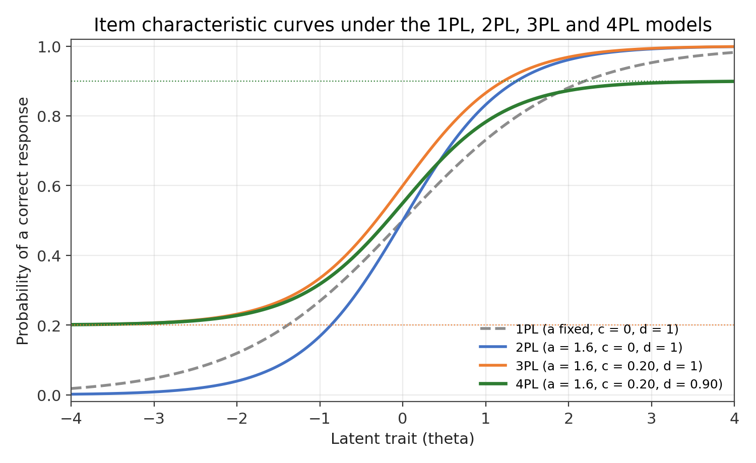
Figure 1. Item characteristic curves under the 1PL, 2PL, 3PL and 4PL models, holding discrimination and location approximately constant to isolate the effect of the asymptotic parameters.

The progression from the 1PL to the 4PL is naturally represented as a chain of nested restrictions, 1PL within 2PL within 3PL within 4PL. Although the models can be arranged in a nested hierarchy of mathematical flexibility, this nesting should not be mistaken for a hierarchy of inferential quality. A model higher in the hierarchy will always achieve a likelihood at least as high as any model nested within it, purely as a mathematical consequence of adding free parameters; whether the additional flexibility is theoretically warranted and empirically justified is a separate question addressed in Section 8.

6. Item Information and Measurement Precision

For the general 4PL model, the item information function is more complex than the familiar 2PL expression, because the response probability is now bounded between ci and di rather than between 0 and 1. Writing Li(theta) for the logistic component of the model,

Li(theta) = 1 / [1 + exp(-ai(theta - bi))], Pi(theta) = ci + (di - ci) Li(theta)

the item information function for the 4PL model is:

Ii(theta) = ai^2 (di - ci)^2 Li(theta)^2 (1 - Li(theta))^2 / [Pi(theta) (1 - Pi(theta))]

which reduces to the familiar 2PL information function, ai^2 Pi(theta)(1 - Pi(theta)), when ci equals zero and di equals one. Figure 2 compares the item information functions implied by 2PL, 3PL and 4PL parameterisations of an otherwise identical item. Introducing a non-zero lower asymptote (3PL) reduces peak information relative to the 2PL, because a non-zero floor compresses the range over which the item can discriminate; introducing a sub-unity upper asymptote (4PL) reduces peak information further, as the compressed ceiling has an analogous effect at the upper end of the continuum.

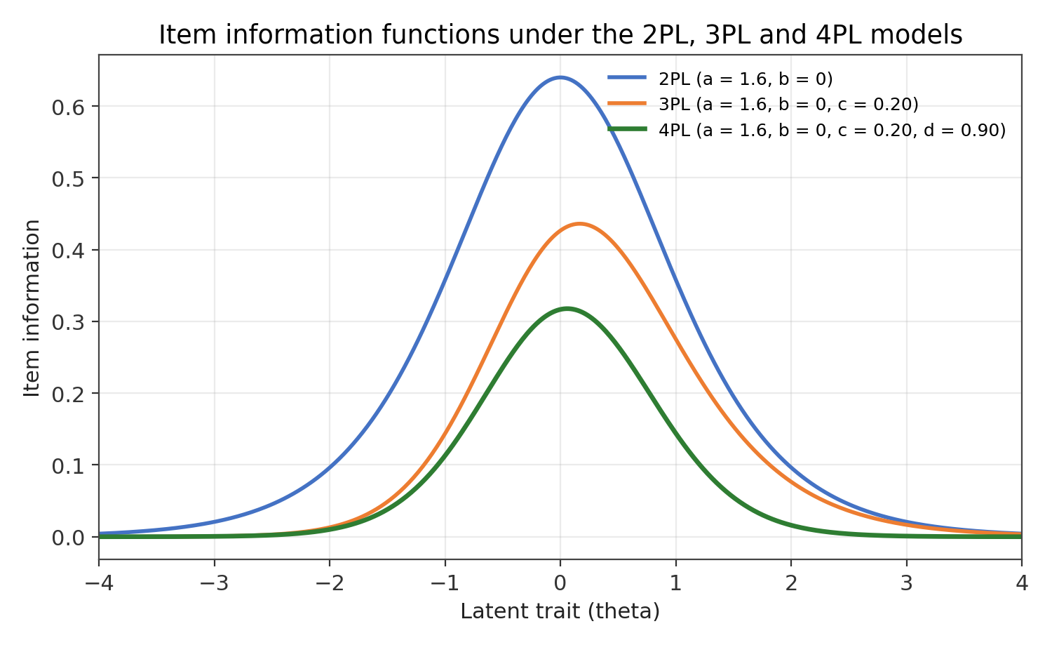
Figure 2. Item information functions under the 2PL, 3PL and 4PL models for an item of fixed discrimination and location, illustrating the reduction in peak information associated with each additional asymptotic parameter.

Researchers should therefore compute and interpret the information function generated by the fitted model actually used, rather than assuming that 2PL information formulae remain applicable once asymptotic parameters are introduced, particularly in computerized adaptive testing, where item selection is explicitly driven by expected information (Section 10.3).

7. Estimation, Identification and Sample Size Requirements

7.1 Identifiability and Boundary Problems

The 3PL and 4PL models contain additional parameters that can be difficult to estimate simultaneously and precisely. Identification difficulties become more likely when samples are small, when items are poorly distributed across the ability continuum, when discrimination is weak, or when the assumed latent-trait distribution is misspecified (Loken and Rulison, 2010; Waller and Feuerstahler, 2017). The parameters ci and di are also bounded, typically satisfying 0 less than or equal to ci, ci less than di, and di less than or equal to 1. Poorly constrained estimation can produce implausible results in which the estimated lower asymptote exceeds the estimated upper asymptote, a configuration that is not substantively coherent. A well-designed IRT platform should implement parameter constraints during estimation and flag, rather than silently correct, any boundary violations, alongside warnings for extreme parameter values, unstable discrimination, large standard errors, and non-convergence.

7.2 Sample Size Considerations

Simulation research indicates that stable recovery of 4PL item parameters generally requires substantially larger samples than the 2PL or 3PL. In an extensive simulation spanning real, realistic and idealised data conditions, Waller and Feuerstahler (2017) found that item parameters and response functions under the 4PL could be recovered accurately using Bayesian modal estimation with samples of approximately 5,000 respondents or more, while person parameters could be recovered in samples of around 1,000 or more under some conditions. Loken and Rulison (2010) similarly showed that, although overall fit improves when the 4PL is used to generate and recover data, inferences at the extremes of the trait continuum are most vulnerable to poor confidence-interval coverage when an over- or under-parameterised model is fitted. These figures are not universal thresholds, since requirements depend on test length and calibration-sample design, but they underline that software support for a model does not, by itself, justify its use.

Table 2 and Figure 3 summarise the approximate growth in the total number of item-level parameters that must be estimated as test length increases across the 2PL, 3PL and 4PL models, illustrating why model complexity, and consequently estimation burden, grows rapidly with test length.

Table 2. Approximate item-level parameter counts under the 2PL, 3PL and 4PL models as a function of test length. Figures exclude latent-distribution and other model-specific parameters.

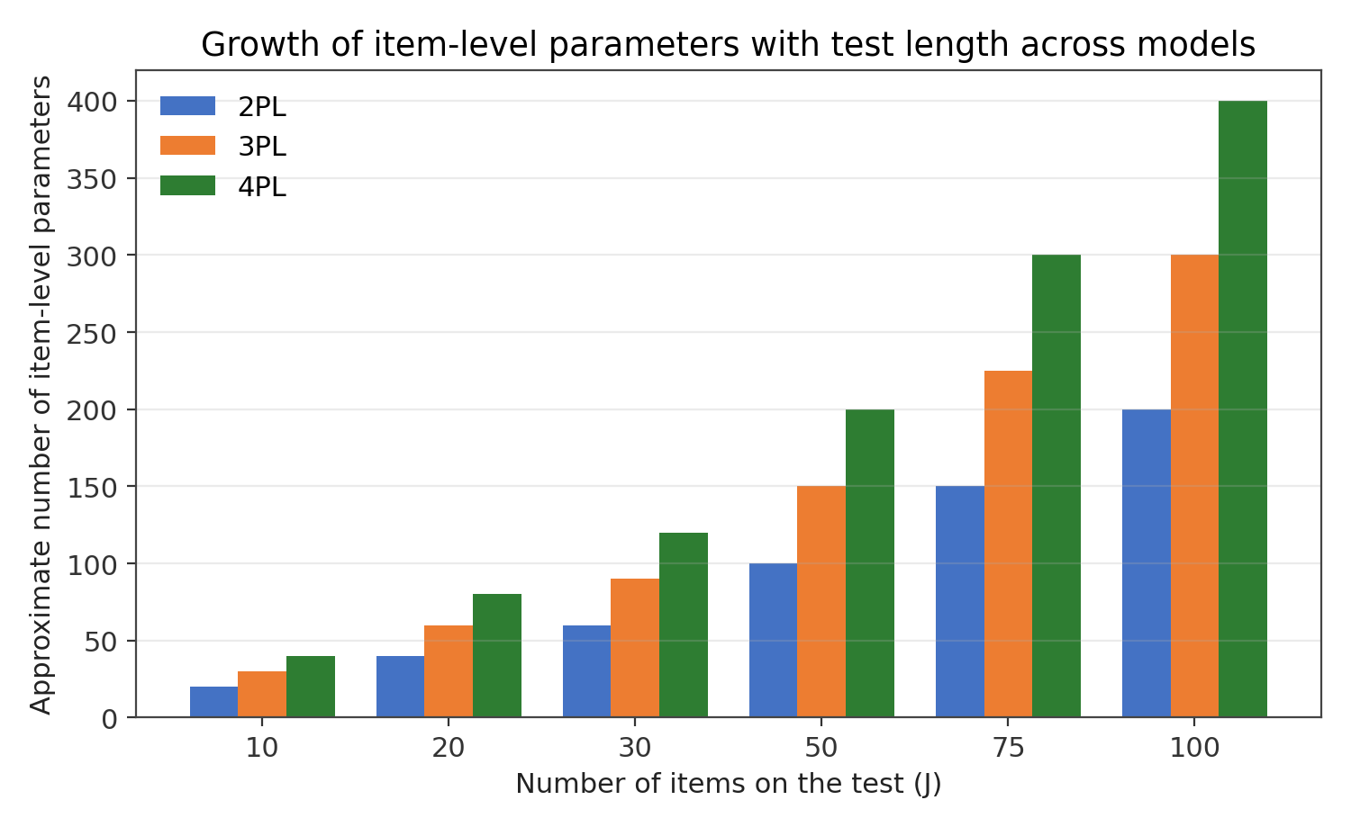
Figure 3. Growth of item-level parameters with test length across the 2PL, 3PL and 4PL models.

8. Model Selection: Fit, Information Criteria and Cross-Validation

8.1 Avoiding the ‘More Parameters Equals a Better Model’ Fallacy

Because the 3PL and 4PL nest the 2PL as a restricted special case, adding parameters can only improve, and will rarely worsen, the raw log-likelihood achieved on the calibration sample. A 4PL model may fit better in likelihood terms while also containing many more free parameters, so better raw fit does not, by itself, establish that the more complex model is preferable for inference or prediction. Researchers should weigh fit improvement against complexity cost using information criteria such as AIC and BIC, which explicitly penalise additional parameters, alongside fit statistics, parameter plausibility, and predictive performance.

8.2 Cross-Validation as a Safeguard

A robust strategy divides data into a calibration sample, used to estimate parameters, and an independent validation sample, used to evaluate predictive performance. If a more complex model produces a substantially better calibration fit but little or no improvement in the validation sample, this pattern is suggestive of overfitting rather than genuine gains in measurement precision (Oladunmoye, & Muhammad, 2024; Oladunmoye, 2015).

9. Differential Item Functioning in the 3PL/4PL Framework

9.1 A Four-Parameter View of DIF

Differential item functioning (DIF) analysis, traditionally focused on discrimination and location, can be naturally extended to the asymptotic parameters of the 3PL and 4PL. For each item, the parameter vector (ai, bi, ci, di) allows a group difference in any component to constitute a distinct form of DIF: a in discrimination, b in location, c in lower-asymptote or pseudo-guessing behaviour, and d in upper-asymptote or slipping and engagement behaviour. This four-parameter view offers a considerably richer picture of measurement fairness than comparisons restricted to item location alone.

9.2 Group-Specific ICCs and Measurement Fairness

A practical way of communicating such differences is to overlay group-specific item characteristic curves. An item might appear acceptable under a conventional 2PL analysis, yet reveal materially different asymptotic behaviour once a 4PL model is fitted separately by group; for example, one group might show an upper asymptote of 0.99 while another shows 0.82. Detecting such a difference is only the first step: the researcher must then investigate plausible explanations, including cultural or linguistic factors, item ambiguity, differential response strategies, or subgroup-specific response processes (Oladunmoye, Agbor, Olabisi, & Oyadeyi, 2024).

10. Applications

10.1 Educational Testing and Multiple-Choice Assessment

The 3PL model has its most natural home in educational and cognitive-ability testing using multiple-choice or similarly structured items, where the possibility of a correct response arising from processes other than full knowledge of the tested construct is well established (Birnbaum, 1968; Hambleton, Swaminathan and Rogers, 1991; Oladunmoye, Enamudu, & Ogbu, 2024).

10.2 Psychological and Clinical Assessment

Application of the 3PL and 4PL to psychological and clinical instruments requires more caution, since many such instruments use self-report items without an objectively correct answer. Reise and Waller (2009), reviewing the use of Item Response Theory in clinical measurement, note that clinical and cognitive measures differ in ways that have direct relevance for model choice; the same caution applies with particular force to guessing- or slipping-type parameters in instruments that do not resemble multiple-choice ability tests. Where the construct lacks a correct answer to guess, the case for a non-zero lower asymptote is weak; where high-trait respondents can plausibly err through inattention or disengagement, particularly in unsupervised digital administration, the case for an upper asymptote is comparatively stronger, though it still requires construct-specific justification rather than automatic application.

10.3 Computerized Adaptive Testing

Computerized adaptive testing selects each subsequent item to maximise expected information at the respondent's current ability estimate. Because ci and di change the shape and peak of the item information function (Section 6), item-selection algorithms calibrated for the 2PL cannot simply be transplanted into a 3PL or 4PL adaptive-testing system; the information function actually implied by the fitted model must drive item selection. A properly implemented 4PL-based algorithm can improve measurement precision relative to a 3PL-based one, though realised benefits depend on estimation quality and the testing programme's specific response conditions.

10.4 Online and Digital Assessment: Response Effort and Response-Time Data

Contemporary online and unproctored digital testing environments introduce response conditions, such as multitasking, distraction, rapid clicking, item abandonment and technical interruption, that differ materially from traditional proctored administration. The upper asymptote of the 4PL model can partially absorb the effects of such behaviour at the item level, but response-process data such as response latency, answer-change patterns, omission rates and interaction logs provide complementary and often more direct evidence about response effort. For example, two respondents with identical estimated ability but markedly different response times on an easy item, say 45 seconds versus 2 seconds, present different candidate explanations for an unexpected error; response-time evidence can help distinguish low ability from rapid or careless responding in a way that the item response function alone cannot. A mature psychometric architecture is therefore likely to combine formal IRT modelling with such process indicators rather than relying on the upper asymptote in isolation.

11. Threats to Valid Interpretation

11.1 Dimensionality and Local Item Dependence

The additional flexibility of the 3PL and, especially, the 4PL should never substitute for addressing multidimensionality. If a test measures a combination of distinct latent dimensions, a flexible unidimensional 4PL model may partially absorb this misspecification into its asymptotic parameters, producing an apparently adequate fit that masks the underlying structure. A related threat arises from local item dependence, where items sharing wording or stimulus material produce correlated residuals that a unidimensional model cannot represent; such dependence can be misattributed to item-specific asymptotic behaviour, distorting c and d estimates. A complete diagnostic workflow should therefore check dimensionality and local dependence before any asymptotic parameters are substantively interpreted.

11.3 Common Misinterpretations

Several misinterpretations of the 3PL and 4PL models recur frequently enough in applied practice to warrant explicit correction.

• The claim that ‘the 3PL measures guessing’ overstates what the model can support. More precisely, the lower asymptote models response probability at low levels of the latent trait, and is commonly, though not universally, interpreted as pseudo-guessing in appropriate testing contexts.
• The claim that ‘the 4PL measures carelessness’ is similarly imprecise. The upper asymptote can model response patterns consistent with slipping or careless error, but the parameter itself does not establish the behavioural cause of that pattern.
• The claim that ‘the 4PL is always better’ than simpler models is incorrect. Additional parameters introduce genuine estimation and identification challenges that can outweigh their theoretical benefits in any given application.
• The claim that ‘a high value of c means respondents guessed’ treats a model parameter as though it were direct observational evidence of guessing behaviour, which it is not.

12. Implications for the PsychtrixWeb Platform

The preceding sections point toward a set of functional requirements for a PsychtrixWeb module supporting 3PL and 4PL analysis. These requirements are organised below under six headings: core modelling, visualisation, diagnostics, fairness analysis, computerized adaptive testing, and reproducibility.

12.1 Core Modelling and Visualisation

The platform should support fitting a 2PL baseline model alongside the 3PL and 4PL, with configurable parameter constraints, for example fixing ci equal to zero for items suspected to have negligible pseudo-guessing, and with the chosen upper-asymptote parameterisation clearly displayed in all output. It should render item characteristic curves with asymptote reference lines, item and test information functions, and conditional standard errors of measurement, in each case for the model actually estimated rather than a generic 2PL approximation.

12.2 Diagnostics

The platform should report convergence status, parameter standard errors, and explicit boundary warnings whenever an estimated lower asymptote meets or exceeds the corresponding upper asymptote, together with item-level and global fit statistics and formal model-comparison output, including log-likelihood, AIC and BIC, for the 2PL, 3PL and 4PL fitted to the same data. Table 3 illustrates the item-level diagnostic panel that should be available for every item in an analysis; the values shown are illustrative only.

Table 3. Illustrative item-level diagnostic panel for a single 4PL item. Values are illustrative only.

12.3 Fairness Analysis Tools

The platform should support differential item functioning analysis across all four item parameters (Section 9.1), including group-specific item characteristic curves that can be overlaid for visual comparison, so that discrimination, location, lower-asymptote and upper-asymptote differences can each be inspected and reported. Table 4 illustrates a recommended item-level reporting format that would allow a research team to record and communicate these results; again, the values are illustrative only.

Table 4. Illustrative multi-item reporting table combining parameter estimates, standard-error reporting and differential item functioning decisions. Values are illustrative only.

12.4 Adaptive Testing and Reproducibility

Where computerized adaptive testing is offered, item-selection routines should compute expected information from the fitted 3PL or 4PL response functions rather than importing 2PL-based heuristics, with stopping rules calibrated accordingly (Section 10.3). A reproducible analysis should also record, and make available for export, the dataset, item coding scheme, model equation and parameterisation, applied constraints, estimation settings, achieved sample size, model-comparison criteria, item-exclusion rules, DIF criteria, and the cross-validation procedure followed.

12.5 Recommended Analytic Workflow

Drawing the preceding requirements together, a recommended end-to-end analytic workflow for a PsychtrixWeb user proceeds through fourteen steps:

1. Upload response data (CSV or XLSX).
2. Define the response coding scheme (typically 0/1).
3. Identify the construct being measured (for example, ability, achievement, or cognitive performance).
4. Assess dimensionality and confirm that a unidimensional latent structure is defensible.
5. Fit a 2PL baseline model.
6. Fit the 3PL model and estimate lower asymptotes.
7. Fit the 4PL model and estimate upper asymptotes.
8. Compare models using likelihood, AIC, BIC and predictive fit.
9. Inspect all estimated item parameters (a, b, c, d) for plausibility.
10. Inspect item characteristic curves for asymptotic behaviour.
11. Inspect item and test information functions for measurement precision.
12. Evaluate differential item functioning across relevant groups.
13. Cross-validate the selected model in an independent sample.
14. Generate a publication-ready methodological report.

A publication-ready report generated from this workflow should allow a researcher to state that a four-parameter model was estimated to evaluate discrimination, location, lower-asymptote and upper-asymptote behaviour; that comparisons were conducted against the 2PL and 3PL; and that item characteristic curves, information functions and differential item functioning were all examined. The report should always state explicitly which parameterisation of the upper asymptote was used, since conventions differ across the literature (Section 4.1).

13. Theoretical and Practical Contribution

The theoretical significance of the movement from the 2PL to the 4PL lies in a single underlying principle: observed response behaviour is probabilistic rather than perfectly deterministic. Respondents with high latent ability can, and periodically do, make errors; respondents with low latent ability can, and periodically do, answer correctly. The 3PL and 4PL models incorporate these realities directly into the mathematical structure of the response function, rather than treating them as unmodelled noise.

For applied researchers, the principal benefit is not added mathematical sophistication for its own sake, but the ability to pose sharper empirical questions: does an item exhibit lower-tail probability consistent with pseudo-guessing; is the lower asymptote substantively plausible; does the item show upper-tail errors consistent with slipping; is the fourth parameter stable across samples; does it improve predictive performance rather than merely calibration fit; and does the item behave consistently across groups? Addressing these questions turns IRT modelling from a technical estimation exercise into an evidence-based practice of measurement evaluation.

14. Conclusion

The 3PL and 4PL models extend the 2PL framework by relaxing the assumption that the probability of a positive response must approach zero and one at the extremes of the latent trait continuum. The 3PL introduces a lower asymptote, commonly interpreted as pseudo-guessing in appropriate testing contexts; the 4PL additionally introduces an upper asymptote, allowing the probability of a correct response to remain below one at very high levels of the latent trait, accommodating response patterns associated with slipping, carelessness or related sources of upper-tail error.

This progression should not be read as an implicit claim that the 2PL is worse than the 3PL, which is in turn worse than the 4PL, in some universal ranking of model quality. Model complexity should be guided by measurement theory and evidence about actual response behaviour, not by the availability of software that can estimate additional parameters. The 4PL can provide genuine flexibility where both guessing and high-ability slipping are theoretically plausible, but its parameters increase estimation complexity and, under many realistic conditions, require substantially larger calibration samples for stable recovery (Waller and Feuerstahler, 2017).

For PsychtrixWeb, the appropriate objective is therefore not simply to add a 4PL option, but to build a genuine IRT model-comparison environment in which researchers can evaluate whether additional parameters are actually warranted by their data and construct: theory, then data, then 2PL, then 3PL, then 4PL, then formal model comparison, diagnostics, and validation.

15. Key Takeaways

1. The 3PL model extends the 2PL by adding a lower asymptote parameter.
2. The lower asymptote is commonly, though not universally, interpreted as pseudo-guessing in appropriate testing contexts.
3. The 4PL model adds an upper asymptote parameter to the 3PL structure.
4. The upper asymptote can accommodate high-ability errors consistent with slipping or careless responding.
5. The fourth parameter does not, by itself, provide a direct diagnosis of individual-level carelessness.
6. The 3PL is most naturally justified for objectively scored, dichotomous, multiple-choice-style tests.
7. The 3PL should not be applied automatically to ordinary psychological self-report items.
8. The 4PL offers greater flexibility than the 3PL, but at the cost of greater estimation demands.
9. Sample-size requirements for stable 4PL parameter recovery can be substantial, plausibly in the low thousands of respondents for item-level recovery.
10. Dimensionality and local item dependence should be investigated before introducing additional unidimensional model complexity.
11. Model selection should weigh fit, information criteria, parameter plausibility and cross-validated predictive performance together.
12. Differential item functioning can, in principle, involve discrimination, location, lower-asymptote or upper-asymptote differences.
13. PsychtrixWeb should allow researchers to compare the 2PL, 3PL and 4PL directly rather than committing them to a single model.
14. The platform's long-term value lies in integrating IRT modelling, diagnostics, differential item functioning analysis, computerized adaptive testing and reproducible reporting within a single coherent workflow.

Suggested citation: Oladunmoye, E. O. (2026). The 3PL and 4PL item response theory models: Modelling guessing, slipping and upper-asymptote behaviour (Extended ed.). PsychtrixWeb Research Notes, 014. Psychtrix Initiative Limited.

References

- Barton, M. A., & Lord, F. M. (1981). An upper asymptote for the three-parameter logistic item-response model (Research Bulletin RR-81-20). Educational Testing Service.
- Birnbaum, A. (1968). Some latent trait models and their use in inferring an examinee's ability. In F. M. Lord & M. R. Novick, Statistical theories of mental test scores. Addison-Wesley.
- Hambleton, R. K., Swaminathan, H., & Rogers, H. J. (1991). Fundamentals of item response theory. Sage.
- Liao, W.-W., Ho, R.-G., Yen, Y.-C., & Cheng, H.-C. (2012). The four-parameter logistic item response theory model as a robust method of estimating ability despite aberrant responses. Social Behavior and Personality: An International Journal, 40(10), 1679-1694.
- Loken, E., & Rulison, K. L. (2010). Estimation of a four-parameter item response theory model. British Journal of Mathematical and Statistical Psychology, 63(3), 509-525.
- Lord, F. M. (1980). Applications of item response theory to practical testing problems. Lawrence Erlbaum Associates.
- Oladunmoye, E. O. (2026a). Item response theory: From observed responses to latent trait measurement. PsychtrixWeb Research Notes, 011.
- Oladunmoye, E. O. (2026b). The Rasch model and 1PL IRT: Understanding item difficulty, person ability, and invariant measurement. PsychtrixWeb Research Notes, 012.
- Oladunmoye, E. O. (2026c). The two-parameter logistic IRT model: Understanding item discrimination, difficulty, and differential item functioning. PsychtrixWeb Research Notes, 013.
- Oladunmoye, E. O. (2026d). Validity in psychological measurement: Beyond reliability and statistical significance. PsychtrixWeb Research Notes, 003.
- Oladunmoye, E. O., (2015). Development and validation of social provision scale on first year undergraduate psychological adjustment. Journal of Education and Practice, 6 (28), 78-90.
- Oladunmoye, E. O., Muhammad T. S., (2024). Development and Validation of Multiple Intelligence Test among emerging adults in the United Kingdom. ISAR Journal of Arts, Humanities and Social Sciences, 2(4), 18-24.
- Oladunmoye, E.O., Agbor, E.C., Olabisi, O.L., and Oyadeyi, J.B., (2024). Estimating measurement invariance on emotional intelligence scale across gender and age among undergraduates in Nigeria. Thinking Skills and Creativity Journal. 7(1),50-60.
- Oladunmoye, E.O., Enamudu, G.P., Ogbu, F. (2024). Comparison of estimate of linear and Equi-percentile CTT equating of WAEC Mathematics test forms 2022 and 2023. International Journal of Humanities Social Science and Management (IJHSSM), 4(3),544-552.
- Oladunmoye, E.O., Enamudu, G.P., Sa'ad, M.T. (2024). A Differential Item Functioning estimate of WAEC Mathematics test form based on gender and age among secondary school students. ISAR Journal of Multidisciplinary Research and Studies, 2(5), 15-21.
- Reise, S. P., & Waller, N. G. (2009). Item response theory and clinical measurement. Annual Review of Clinical Psychology, 5, 27-48.
- Waller, N. G., & Feuerstahler, L. M. (2017). Bayesian modal estimation of the four-parameter item response model in real, realistic, and idealized data sets. Multivariate Behavioral Research, 52(3), 350-370.
Suggested citation
Oladunmoye, E. O. (2026). The 3PL and 4PL Item Response Theory Models. PsychtrixWeb Research Note, 015. Psychtrix Initiative Limited. https://www.psychtrixweb.online/research-notes/015-abstract-3Discuss this Research Note
Scholarly comments are welcome from anyone — no account required. Contributions are moderated before they appear.
No comments yet. Start the scholarly discussion below.