The Two-Parameter Logistic IRT Model: Understanding Item Discrimination, Difficulty, and Differential Item Functioning

1. Introduction

Item Response Theory (IRT) provides a framework for modelling the probability that a person will produce a particular response to an item as a function of two things: the person's location on an underlying latent trait, and the characteristics of the item itself. As established in Research Note 011 on the foundations of IRT (Embretson & Reise, 2000), the approach moves beyond the classical assumption that all relevant information about a person's measurement status can be adequately summarised by a raw total score.

Research Note 012 subsequently introduced the Rasch model as a particularly important restricted IRT model, in which every item is constrained to share a common discrimination parameter under the conventional logistic parameterisation (Baker & Kim, 2004). The present note introduces the two-parameter logistic model, commonly abbreviated as the 2PL model. The defining feature of the 2PL is the estimation of two item parameters for every item: an item difficulty, or location, parameter, and an item discrimination parameter. The model therefore permits items to differ not only in where they are located along the latent continuum, but also in how sharply they distinguish among respondents situated around that location.

This flexibility is the single most important conceptual departure from the Rasch/1PL family, and it carries consequences that extend through nearly every stage of psychometric practice, from item calibration and scale development to fairness analysis and computerised adaptive testing (Oladunmoye, 2026b). The sections that follow build up the 2PL model systematically, from its basic equation to its role in a fully specified PsychtrixWeb analytic workflow (Oladunmoye, 2026c).

2. The Basic 2PL Model

For dichotomous item responses, the 2PL model is commonly expressed as the probability that a randomly selected respondent with latent trait level theta will produce a positive response (X = 1) to item i:

P(Xi = 1 | θ) = exp[ai(θ - bi)] ÷ {1 + exp[ai(θ - bi)]}

where Xi is the response to item i, θ (theta) is the respondent's latent trait level, ai is the discrimination parameter for item i, and bi is the difficulty, or location, parameter for item i. An algebraically equivalent and more commonly used formulation is:

P(Xi = 1 | θ) = 1 ÷ {1 + exp[-ai(θ - bi)]}

The two parameters serve distinct functions within the model. The discrimination parameter, ai, describes how sharply the item distinguishes between respondents; the location parameter, bi, describes where on the latent continuum the item is centred. This separation of roles is summarised concisely as: ai governs how sharply an item discriminates, while bi governs where the item is located.

3. The Difference Between the 1PL and 2PL Models

The distinction between the one-parameter and two-parameter logistic models can be represented directly by comparing their equations. Under the 1PL, or Rasch, model:

P(Xi = 1 | θ) = 1 ÷ {1 + exp[-(θ - bi)]}

Here the discrimination parameter is fixed at a common value (conventionally 1) across all items. Under the 2PL model, by contrast:

P(Xi = 1 | θ) = 1 ÷ {1 + exp[-ai(θ - bi)]}

the discrimination parameter is allowed to vary freely from item to item, such that a1 does not necessarily equal a2, which does not necessarily equal a3, and so on. This single change makes the 2PL model considerably more flexible than the 1PL model, at the cost of estimating one additional parameter for every item in the instrument. Table 1 summarises the principal differences between the two models.

Table 1. Principal differences between the 1PL (Rasch) and 2PL models.

4. Why Add a Discrimination Parameter?

Consider two items that share the same difficulty, b1 = b2 = 0, but differ in discrimination, with a1 = 0.5 and a2 = 2.0. Both items are located at approximately the same point on the latent continuum, yet Item 2 possesses a much steeper response curve than Item 1. As a consequence, around the shared location, a small change in θ produces a considerably larger change in response probability for Item 2 than for Item 1. Figure 1 illustrates this contrast directly.

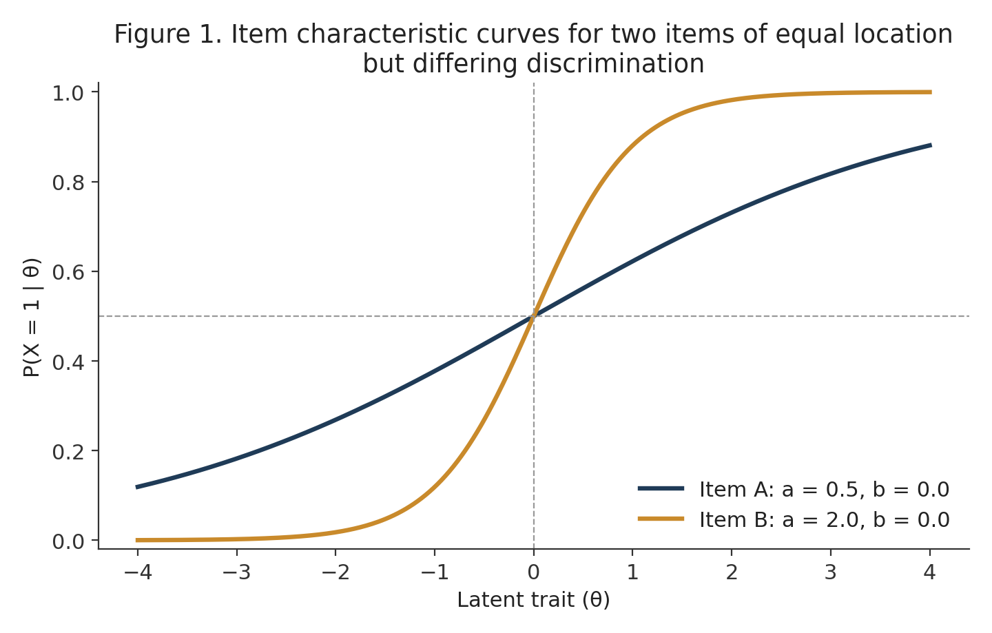
Figure 1. Item characteristic curves for two items of equal location but differing discrimination. The steeper curve (Item B) provides more information near θ = 0.

The higher-discrimination item therefore provides more information about differences between respondents in the region of the trait continuum surrounding its location. This is the central practical motivation for allowing discrimination to vary: some items are simply more sensitive indicators of standing on the latent trait than others.

5. Item Difficulty in the 2PL Model

The parameter bi represents the location of item i on the latent trait scale. For the standard 2PL model, without a guessing parameter, the following identity holds at the point where θ equals bi:

P(Xi = 1 | θ = bi) = 0.50

Thus, bi is the trait level at which the probability of a positive response is approximately fifty per cent. This property makes the interpretation of bi relatively straightforward within the standard 2PL formulation. For psychological self-report instruments, however, the term item difficulty can be misleading. An item concerning depressive symptoms, for example, is not "difficult" in the sense used in educational testing; it instead represents a symptom-endorsement location on the latent continuum. For this reason, researchers working with psychological and attitudinal measures frequently prefer the term item location to item difficulty when describing bi.

6. Item Discrimination

The parameter ai represents the discrimination of item i and determines the steepness of the item's characteristic curve. A relatively low discrimination value produces a comparatively flat curve, whereas a relatively high discrimination value produces a comparatively steep curve. Higher discrimination therefore means that the item is more sensitive to differences in trait level in the vicinity of its location, while changes in bi simply shift the curve horizontally along the trait continuum without altering its steepness.

7. The Item Characteristic Curve

The item characteristic curve (ICC) is among the most important visual representations used in IRT. It plots the probability of a positive response, P(Xi = 1), against the latent trait, θ, and thereby shows how response probability changes across the entire trait continuum. For the 2PL model, two features of the curve merit particular attention: its horizontal location, determined primarily by bi, and its steepness, determined by ai. In short, bi governs location and ai governs steepness.

8. High Discrimination Does Not Automatically Mean a Good Item

This is an important psychometric caution. A high discrimination parameter is not equivalent to construct validity. An item may discriminate sharply for several reasons, only some of which reflect a genuinely strong relationship with the intended construct: it may be strongly related to the construct being measured, worded with unusual clarity, or reliant on a distinctive cue that respondents latch onto; alternatively, it may measure only a narrow subdimension, be affected by wording effects unrelated to the construct, function differently across subgroups (see Section 19 on DIF), or reflect an unintended secondary construct (Oladunmoye, Enamudu, & Sa'ad, 2024).

It follows that high discrimination does not automatically indicate a high-quality item. Statistical discrimination must always be interpreted alongside substantive content review and independent validity evidence, rather than treated as a self-sufficient indicator of item quality.

9. The 2PL Model and the Latent Trait

The 2PL model assumes that the observed response is related to an underlying latent variable. For respondent p, θp represents that person's location on the latent continuum. Examples of latent traits commonly modelled with the 2PL include anxiety, depression, resilience, cognitive ability, academic achievement, self-efficacy, psychological wellbeing, attitudes, and personality dimensions. The model transforms discrete item responses into probabilistic information about a person's location on this underlying continuum.

10. Local Independence and Unidimensionality

The 2PL model typically assumes local independence: once the latent trait is held constant, responses to different items are conditionally independent of one another, P(X1, X2, ... , Xn | θ) = Π P(Xi | θ) for i = 1 to n. Local dependence can arise when items share highly similar wording, when one item's content depends on another, when items share a common stimulus, or when respondents adopt a particular response strategy across a set of items; it can inflate apparent information and distort standard errors, so 2PL analysis should never be interpreted in isolation from local-dependence diagnostics.

A conventional 2PL model also assumes a single dominant latent dimension. Suppose a questionnaire is intended to measure academic self-efficacy, but several items primarily capture test anxiety instead; the assumption of unidimensionality then becomes questionable, creating a direct methodological link to Research Note 006 on dimensionality (Reckase, 2009; Oladunmoye, 2026a). A useful analytic sequence proceeds from construct definition, to dimensionality assessment, to IRT model selection, to item calibration.

11. Item Information and Maximum Information

An important consequence of allowing discrimination to vary across items is that item information varies substantially as well. For a dichotomous 2PL item, information is given by Ii(θ) = ai² × Pi(θ) × [1 - Pi(θ)], where the squared discrimination parameter is critical: as ai increases, the maximum information the item can supply increases as the square of that value, so even modest gains in discrimination can translate into substantial gains in information.

Maximum item information occurs at the item's own location, where θ is approximately equal to bi and Pi = Qi = 0.50, giving Ii(bi) = ai² ÷ 4. This demonstrates mathematically why discrimination matters so much for precision. If a = 1.0, the maximum item information is 0.25; if a = 1.5, it rises to 0.563; if a = 2.0, it reaches 1.00; and if a = 2.5, it reaches 1.563, at which point local dependence should be checked. An item with a = 2.0 therefore provides four times the maximum information of an item with a = 1.0, around its own location.

12. Test Information

Individual item information functions can be summed directly to obtain the test information function (TIF):

IT(θ) = Σ Ii(θ) for i = 1 to n

Research Note 011 introduced information as a fundamental feature of IRT; the present note extends that concept by demonstrating that the discrimination parameter strongly determines how much information any individual item can contribute to the total.

13. Standard Error of Measurement in IRT

A commonly used relationship links the test information function directly to the conditional standard error of the ability estimate:

SE(θ) = 1 ÷ √[IT(θ)]

It follows that as test information increases, the standard error of measurement decreases, and vice versa. This means that the precision of measurement varies across the latent trait continuum: a test may measure respondents very precisely around θ = 0 while providing considerably less precision at θ = 2.5. This is one of the principal differences between IRT-based measurement and a single global reliability coefficient, which necessarily averages precision across the entire range of the trait.

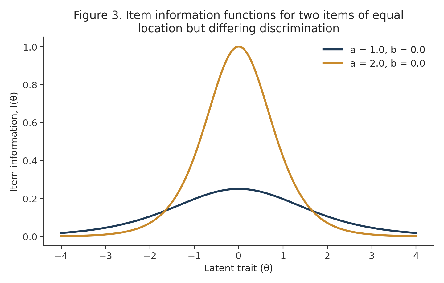
Figure 3. Item information functions for two items of equal location but differing discrimination. Information peaks at the item's own location and scales with a².

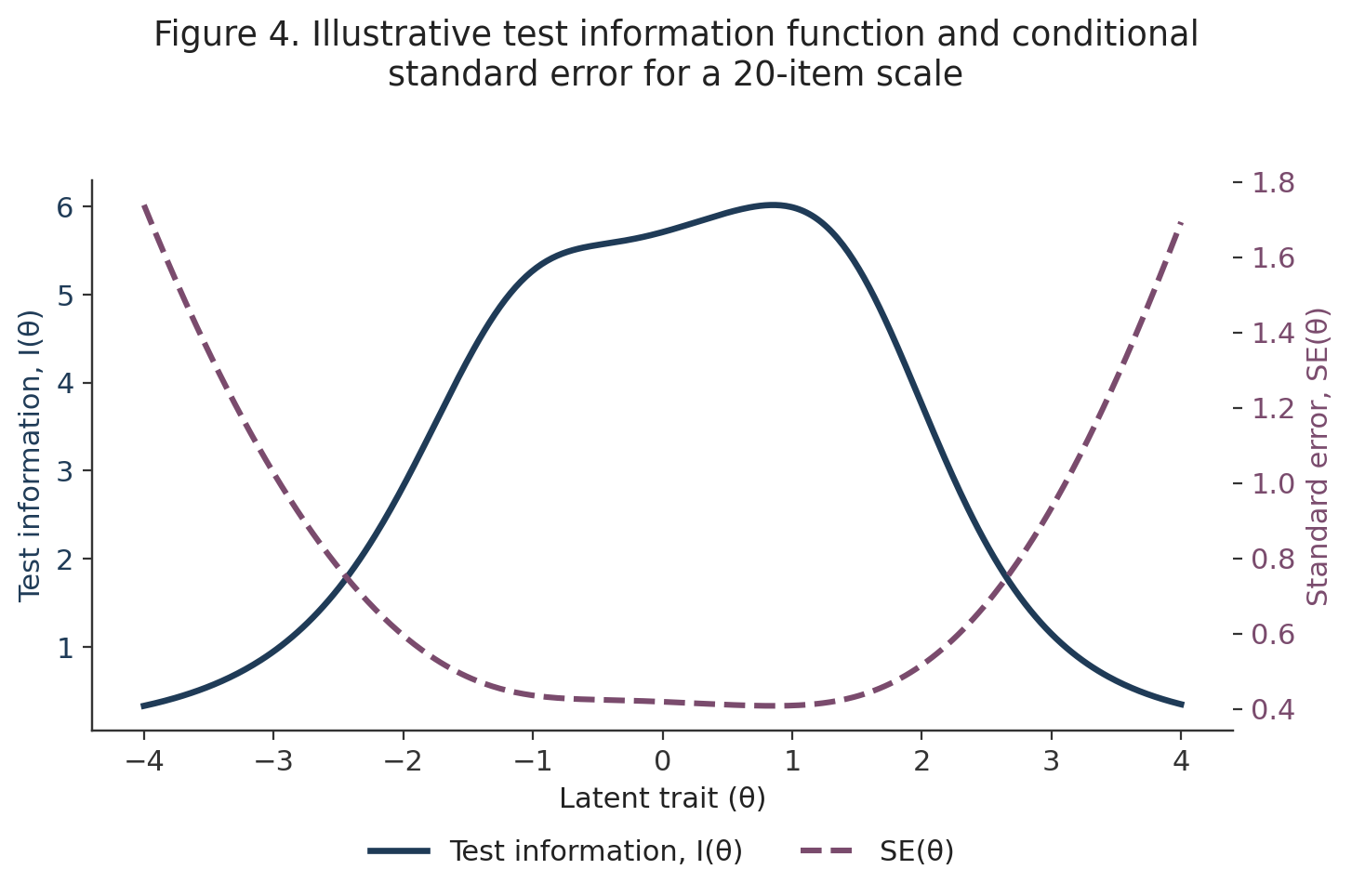
Figure 4. Illustrative test information function (solid line) and conditional standard error (dashed line) for a 20-item scale. Precision is greatest, and the standard error smallest, near the centre of the trait distribution.

14. Estimating Person Ability

Discrimination is sometimes loosely compared with a classical item-total correlation, but the analogy should never be treated as a strict equivalence: an item-total correlation is a sample-dependent statistic drawn from Classical Test Theory, whereas the 2PL discrimination parameter is a model-based parameter describing the relationship between response probability and the latent trait itself, and the two should not be reported as equivalent.

Unlike the Rasch model, the 2PL model generally cannot rely on the raw score alone to identify a person's latent trait estimate, because items carry different discrimination values: two respondents with identical raw scores can have different likelihood functions if they answered highly discriminating items differently from weakly discriminating items. Consider two respondents who both obtain a raw score of X = 15, one by answering correctly on highly discriminating items and the other on weakly discriminating items; under classical test theory these respondents would be treated identically, but under 2PL IRT their response patterns contain different amounts of information about their respective latent trait estimates, θA and θB, which may differ meaningfully. This is a central conceptual advantage of the IRT framework over a simple total-score approach. The latent trait estimate is instead obtained through an appropriate estimation method, such as maximum likelihood, expected a posteriori, maximum a posteriori, or another Bayesian or marginal method, with the most appropriate choice depending on the measurement design and intended application.

15. Identification and Scaling

IRT parameters require a defined scale before they can be interpreted. A common convention sets θ to follow a standard normal distribution, θ ~ N(0, 1), such that its expected value is zero and its variance is one; item parameters are then estimated relative to this latent metric. Some software also incorporates a scaling constant, commonly denoted D, so that the probability function appears as P(Xi = 1 | θ) = 1 ÷ {1 + exp[-D × ai(θ - bi)]}. Different conventions can produce different numerical values for discrimination even when the underlying item behaviour is identical, so researchers should always report the model, link function, parameterisation, and estimation method used, and should never compare a-parameters across studies or software packages without first checking which convention was used. This is a frequent and entirely avoidable source of reporting error in the applied literature.

16. The 2PL Model Versus the Rasch Model, and the Cost of Flexibility

The distinction introduced in Research Note 012 can now be stated more explicitly. The 2PL model can be understood as a direct relaxation of the common-discrimination restriction that defines the Rasch model. Where the Rasch model asks whether a single, shared discrimination value is a defensible representation of every item in an instrument, the 2PL model permits discrimination to vary freely, at the cost of the strong invariance properties that make the Rasch model attractive to many measurement theorists. This flexibility is not obtained without cost: when every item receives its own discrimination parameter, the overall model contains more parameters that must be estimated from the same data, increasing estimation demands, sample-size requirements, parameter instability, and sensitivity to model misspecification. A researcher should therefore never adopt the 2PL model simply because it is perceived as "more advanced" than the Rasch model; the choice should instead be driven by measurement theory and empirical evidence, as elaborated in Section 33.

17. Model-Data Fit and Item-Level Diagnostics

A model can appear statistically attractive while remaining substantively problematic. Model evaluation should therefore consider global fit, item-level fit, residual behaviour, dimensionality, local dependence, parameter plausibility, information, and substantive item content together; a single fit statistic should never be treated as definitive evidence that a scale is psychometrically sound. At the item level, warning signs include excessive residuals, poor item fit, unstable discrimination estimates, unexpected response patterns, and anomalous item characteristic curves. A problematic item should be investigated rather than automatically deleted; the decision to retain, revise, or remove it should weigh statistical evidence together with content, theory, and validity considerations.

18. Diagnostic Signatures: Low and Negative Discrimination

Suppose an item has ai = 0.15. Such an item has a relatively flat item characteristic curve, and its response probability changes only slowly as θ changes, so it may provide little information for distinguishing between respondents at nearby trait levels. Possible explanations include ambiguous wording, weak relevance to the intended construct, multidimensionality, excessive measurement noise, poor response categories, or unusual subgroup functioning.

A more urgent diagnostic condition arises when ai is negative, indicating that higher trait levels are associated with a lower probability of a positive response, the opposite of the intended relationship. This may occur because an item is reverse-worded and has not been properly recoded, because it measures the opposite construct to that intended, because the latent dimension has been incorrectly specified, or because of substantial multidimensionality. Suppose the intended item reads, "I feel capable of managing difficult situations," but the researcher accidentally codes the response direction incorrectly during data entry; the fitted model may then detect a < 0 for that item, providing a useful data-quality diagnostic in its own right. PsychtrixWeb should therefore include a pre-analysis option allowing researchers to identify and reverse-score items prior to calibration.

Automated diagnostic flags

Table 3 summarises a proposed set of automated diagnostic flags that a mature 2PL implementation should surface to the researcher as prompts for investigation, rather than as automatic deletion rules.

Table 3. Proposed automated psychometric flags for a PsychtrixWeb 2PL module.

19. The 2PL Model and Differential Item Functioning

The 2PL model is also central to investigating Differential Item Functioning (DIF). Suppose two groups share the same latent trait level, θ = 1.0. If the probability of endorsing a particular item differs systematically between the groups at this shared trait level, the item may be functioning differently across groups. DIF can arise through differences in bi, through differences in ai, or through both simultaneously. Group differences of this kind may take the form of uniform DIF, in which items differ in location, or nonuniform DIF, in which items differ in discrimination across groups. This provides a direct bridge to Research Note 010 on DIF (Holland & Wainer, 1993).

20. Uniform Versus Nonuniform DIF

Suppose bA does not equal bB, while aA equals aB. In this case the groups differ only in item location, which resembles uniform DIF: the item is consistently harder, or easier, for one group across the entire trait range. Alternatively, suppose aA does not equal aB; here the item discriminates differently across groups, which represents nonuniform DIF. The practical distinction matters because the same item can be equally difficult for two groups at some trait levels while behaving quite differently at others; a summary comparison of group means would miss this pattern entirely (Oladunmoye, Enamudu, & Ogbu, 2024).

Table 4. Uniform, nonuniform, and combined Differential Item Functioning under the 2PL model.

21. The 2PL Model and Measurement Fairness

DIF analysis should never be confused with a simple comparison of group means. A finding that the mean trait level of Group A exceeds that of Group B does not, by itself, establish item bias. DIF concerns the functioning of an item conditional on the underlying trait, not the overall distribution of the trait across groups. It follows that a group difference is not equivalent to DIF, and that the absence of detected DIF is not complete proof of fairness. This distinction is fundamental to responsible practice in psychological measurement.

22. The 2PL Model and Cross-Cultural Assessment

The issue of fairness becomes especially important when instruments are translated or transported across populations. Suppose an anxiety item has a = 1.7 and b = 0.8 in Population A, but after adaptation for Population B produces a = 0.9 and b = 0.2. This change may indicate meaningful differences in item functioning, but the researcher must determine whether it reflects translation quality, cultural interpretation, genuine construct differences, sampling variation, or authentic psychometric differences between populations. IRT statistics identify a measurement phenomenon; they do not, on their own, explain its cultural cause.

23. The 2PL Model in Psychological Scale Development

A practical scale-development workflow situates the 2PL model within a broader sequence of decisions rather than treating it as a stand-alone analysis. A recommended sequence proceeds as follows: (1) construct definition; (2) item generation; (3) content validation; (4) pilot data collection; (5) dimensionality assessment; (6) 2PL calibration; (7) item discrimination review; (8) item location review; (9) item information review; (10) DIF analysis; (11) item refinement; and (12) confirmation of parameter stability in an independent validation sample.

This sequence is considerably more defensible than selecting items exclusively on the basis of corrected item-total correlations, since it incorporates dimensionality, information, and fairness evidence alongside discrimination and location.

24. Short-Form Development, Item Selection, and Adaptive Testing

The 2PL model is particularly useful when developing short forms of longer instruments. Suppose a 40-item scale must be reduced to 12 items; a researcher should not simply retain the items with the highest discrimination values. The selected items should jointly provide adequate construct coverage, appropriate location coverage across the trait range, high information where the target population is concentrated, acceptable DIF characteristics, and acceptable overall precision. For example, if the target population is concentrated around θ = 1.5, an item with b = 1.5 and a = 2.0 may be highly informative for this population, whereas an item with b = -2.0 may contribute very little, regardless of its discrimination value. Short-form optimisation is therefore not equivalent to ranking items by discrimination alone; a and b must always be considered jointly.

The same logic underlies computerised adaptive testing (CAT). Suppose the current trait estimate for a respondent is theta-hat equal to 0.8; the CAT engine evaluates the available item bank, selects an item expected to provide high information around that estimate, and updates the estimate once the respondent answers. This cycle repeats until the standard error of the trait estimate falls below a predefined threshold, or another stopping rule, such as a fixed maximum test length, is reached.

25. Proposed PsychtrixWeb 2PL Engine

A mature PsychtrixWeb implementation should allow the researcher to specify, at minimum, four categories of input and output. Under Data, the researcher specifies the respondent identifier, item variables, missing-data codes, reverse-scored items, and demographic variables. Under Model, the researcher specifies the 2PL model, the estimation method, the latent-trait scaling convention, convergence criteria, and starting values. Under Outputs, the engine returns discrimination and location parameters with their standard errors, item characteristic curves, item and test information functions, conditional standard error, item fit statistics, and person estimates. Under Fairness, the engine conducts DIF analysis by sex or gender where substantively appropriate, and by age, education, geographic group, language, or any other researcher-defined grouping variable.

26. Proposed PsychtrixWeb 2PL Dashboard

A publication-oriented dashboard could display, side by side, the item characteristic curves for a selected subset of items, the test information function overlaid with its conditional standard error, a summary table of item parameters and fit statistics, and a fairness panel summarising any flagged DIF results. The illustrative values used throughout this note, including those in the accompanying figures, are not empirical results drawn from any real dataset. The five diagnostic flags introduced earlier (Table 3) should be presented within this interface as prompts for substantive investigation, not as rules that trigger automatic item deletion, reflecting the broader principle that statistical evidence must always be interpreted alongside content, theory, and independent validity evidence.

27. Sample Size, Parameter Stability, and Replication

There is no universal sample size that guarantees a successful 2PL analysis. Requirements depend on the number of items and parameters, the shape of the trait distribution, the range of discrimination and difficulty values, the amount of missing data, and the estimation method. Because the 2PL model estimates more parameters than the Rasch or 1PL model, it generally requires more information for stable calibration, so researchers should justify their sample size with reference to their specific design rather than an arbitrary universal threshold.

A useful validation strategy compares parameter estimates obtained from independent samples. Suppose a calibration sample of N = 500 produces a discrimination estimate of 1.80 for an item, while an independent validation sample of N = 500 produces an estimate of only 0.72 for the same item. Such a dramatic change should prompt investigation of parameter instability, with possible explanations including sampling differences, multidimensionality, local dependence, DIF, or model misspecification. Psychometric parameters are model-based estimates obtained from particular data under particular assumptions, not immutable properties of items, and their credibility increases with replication rather than with confidence placed in any single sample. A strong scale-development programme therefore involves calibration, cross-validation, external validation, subgroup analysis, and, where appropriate, longitudinal evaluation.

28. The 2PL Model, Validity, and Reliability

IRT does not replace validity theory. An instrument may possess excellent 2PL parameters and still fail to demonstrate adequate content, construct, criterion-related, or consequential validity. This reinforces the principle established in Research Note 003 (Messick, 1995; Oladunmoye, 2015; Oladunmoye, & Muhammad 2024): psychometric modelling is evidence for validity, not validity itself.

Traditional reliability coefficients remain useful in many contexts, but the 2PL model provides a more conditional perspective on measurement precision. Rather than asking only how reliable the scale is overall, the researcher can ask at which levels of the latent trait the scale provides the greatest precision. Suppose, for example, that test information at θ = -2 is 2.5, at θ = 0 is 15.0, and at θ = 2 is 4.0; the scale is then considerably more precise around θ = 0 than at either extreme. A single alpha coefficient cannot communicate this pattern of conditional precision.

29. A Worked Psychometric Interpretation Example

Suppose a 20-item anxiety measure produces discrimination values ranging from 0.40 to 2.10, with most items located between b = -1.5 and b = 1.5. The person-item distribution indicates that most respondents are concentrated around θ = 0, and the resulting test information function peaks between θ = -0.5 and θ = 0.5, broadly consistent with the illustrative pattern shown in Figure 4. A reasonable interpretation of these results might read as follows: the scale provides its greatest measurement precision around average levels of anxiety, while precision decreases towards the extreme ends of the latent continuum, and several highly discriminating items contribute substantially to information around the central trait region. This style of interpretation is considerably more informative than reporting a single figure, such as Cronbach's alpha of .91, in isolation.

30. Common Errors in 2PL Interpretation

Table 7 summarises four errors that recur frequently in applied reporting of 2PL results, alongside the corrected interpretation in each case.

Table 7. Common errors in the interpretation of 2PL item parameters.

31. Research Design and Psychometric Software Design

2PL analysis supports several distinct research designs: cross-sectional scale development, moving from pilot data through calibration to item refinement; cross-cultural validation, moving from the original scale through translation and calibration to DIF analysis; longitudinal assessment, examining whether the measurement model remains stable across successive occasions; and clinical screening, identifying where the instrument provides adequate precision for clinically relevant regions of the trait continuum.

A sophisticated software system should not expose the 2PL model as a single button labelled "2PL". Instead, the interface should guide the researcher through the underlying logic in a defensible sequence: construct, data, response format, dimensionality, model choice, calibration, diagnostics, fairness, refinement, and finally report. This sequence is considerably more defensible than a single-click model-fitting tool, since it makes explicit each decision a competent researcher would otherwise make manually.

32. A Reproducible Workflow and Implications for PsychtrixWeb

An automated report generated from the PsychtrixWeb 2PL engine should contain six sections: model specification (the logistic form, response coding, latent-trait scaling, and estimation procedure); item parameters (discrimination, location, and standard errors); graphical analysis (item characteristic curves, item and test information, and conditional standard error); diagnostics (item fit, residuals, local dependence, and convergence); fairness (DIF statistics, group-specific curves, and flagged items); and interpretation (measurement precision, item coverage, limitations, and recommendations). A reproducible analysis should record data, coding decisions, the model specified, the estimation method, the diagnostics conducted, and the decision rules applied, as a single documented package, so that a reader can trace which items were analysed, which were reverse-scored, which estimation method and parameterisation were used, and which items were removed and why.

The 2PL engine can become a central component of PsychtrixWeb's broader IRT architecture. The recommended progression moves from Classical Test Theory, through the Rasch or 1PL model, through the 2PL model, and onward to the three-parameter and four-parameter logistic models, with DIF analysis, information functions, and computerised adaptive testing operating across the entire environment, allowing researchers to compare models directly rather than being confined to a single psychometric framework by default.

33. Model Selection Should Be Theory-Driven

Table 9 summarises a useful decision rule for selecting among the Rasch/1PL, 2PL, 3PL, and 4PL models.

Table 9. A theory-driven decision rule for selecting among common dichotomous IRT models.

The choice among these models should always rest on measurement objective, theory, and data considered together, rather than on model complexity alone. The most important conceptual distinction between Research Note 012 and the present note can be stated concisely: the Rasch model asks whether a common-discrimination measurement model is defensible for a given instrument, whereas the 2PL model permits discrimination to vary across items. The latter provides greater flexibility, but it also changes the underlying theoretical structure of measurement, so flexibility is not equivalent to automatic superiority.

34. Conclusion

The two-parameter logistic model represents an important advancement beyond the restricted 1PL and Rasch framework, because it permits items to differ in both location and discrimination, following its fundamental equation P(Xi = 1 | θ) = 1 ÷ {1 + exp[-ai(θ - bi)]}. The two parameters play complementary roles: bi describes where an item functions along the latent continuum, while ai describes how sharply the item functions at that location. This allows researchers to identify items that are highly informative at specific regions of the trait continuum and provides a considerably more flexible representation of empirical item behaviour than the Rasch model allows.

However, the 2PL model should never be treated as automatically superior to Rasch measurement. Its additional flexibility introduces greater parameter complexity and relaxes some of the strong restrictions that give the Rasch framework its distinctive invariance properties, so model selection should be driven by measurement theory, substantive objectives, and empirical evidence rather than a general preference for more complex models. For PsychtrixWeb, the 2PL module should become more than a parameter-estimation function: it should integrate calibration, item and test information, DIF analysis, model diagnostics, and automated reporting within a single coherent workflow, moving researchers from simple questionnaire scoring towards genuinely information-based psychological measurement.

35. Key Takeaways

• The 2PL model estimates both item location (b) and item discrimination (a) for every item, with b marking an item's position on the trait continuum and a governing the steepness of its response curve.
• Higher discrimination generally produces greater information around an item's own location, but is more flexible, and more parameter-hungry, than the common-discrimination Rasch/1PL model.
• High discrimination does not automatically establish validity, and negative discrimination should always trigger substantive and data-quality investigation rather than automatic deletion.
• Differential Item Functioning can involve differences in item location, discrimination, or both simultaneously, and is distinct from a simple difference in group means.
• Item and test information show where a scale measures most precisely across the trait continuum; a single reliability coefficient cannot represent this conditional precision.
• PsychtrixWeb should integrate 2PL calibration with information functions, DIF analysis, diagnostics, visualisation, and reproducible reporting within a single workflow.

Suggested Citation

Oladunmoye, E. O. (2026). The two-parameter logistic IRT model: Understanding item discrimination, difficulty, and differential item functioning. PsychtrixWeb Research Notes, 013. Psychtrix Initiative Limited.

References

- Baker, F. B., & Kim, S.-H. (2004). Item response theory: Parameter estimation techniques (2nd ed.). CRC Press.
- Birnbaum, A. (1968). Some latent trait models and their use in inferring an examinee's ability. In F. M. Lord & M. R. Novick, Statistical theories of mental test scores (pp. 397 to 479). Addison-Wesley.
- Embretson, S. E., & Reise, S. P. (2000). Item response theory for psychologists. Lawrence Erlbaum Associates.
- Hambleton, R. K., & Jones, R. W. (1993). Comparison of classical test theory and item response theory and their applications to test development. Educational Measurement: Issues and Practice, 12(3), pp. 38 to 47.
- Holland, P. W., & Wainer, H. (Eds.). (1993). Differential item functioning. Lawrence Erlbaum Associates.
- Lord, F. M. (1980). Applications of item response theory to practical testing problems. Lawrence Erlbaum Associates.
- Messick, S. (1995). Validity of psychological assessment: Validation of inferences from persons' responses and performances as scientific inquiry into score meaning. American Psychologist, 50(9), pp. 741 to 749.
- Oladunmoye, E. O. (2026a). Item response theory: From observed responses to latent trait measurement. PsychtrixWeb Research Notes, 011.
- Oladunmoye, E. O. (2026b). The Rasch model and 1PL IRT: Understanding item difficulty, person ability, and invariant measurement. PsychtrixWeb Research Notes, 012.
- Oladunmoye, E. O. (2026c). The two-parameter logistic IRT model: Understanding item discrimination, difficulty, and differential item functioning. PsychtrixWeb Research Notes, 013.
- Oladunmoye, E. O., (2015). Development and validation of social provision scale on first year undergraduate psychological adjustment. Journal of Education and Practice, 6 (28), 78-90.
- Oladunmoye, E. O., Muhammad T. S., (2024). Development and Validation of Multiple Intelligence Test among emerging adults in the United Kingdom. ISAR Journal of Arts, Humanities and Social Sciences, 2(4), 18-24.
- Oladunmoye, E.O., Enamudu, G.P., Ogbu, F. (2024). Comparison of estimate of linear and Equi-percentile CTT equating of WAEC Mathematics test forms 2022 and 2023. International Journal of Humanities Social Science and Management (IJHSSM), 4(3),544-552.
- Oladunmoye, E.O., Enamudu, G.P., Sa'ad, M.T. (2024). A Differential Item Functioning estimate of WAEC Mathematics test form based on gender and age among secondary school students. ISAR Journal of Multidisciplinary Research and Studies, 2(5), 15-21.
- Reckase, M. D. (2009). Multidimensional item response theory. Springer.
- Reise, S. P., & Waller, N. G. (2009). Item response theory and clinical measurement. Annual Review of Clinical Psychology, 5, pp. 27 to 48.
- Samejima, F. (1969). Estimation of latent ability using a response pattern of graded scores. Psychometrika Monograph Supplement, No. 17. Psychometric Society.
- van der Linden, W. J. (Ed.). (2018). Handbook of item response theory: Models (Vol. 1). Chapman & Hall / CRC.